協調フィルタリングモジュール collab と推奨システム D-Recommend

協調フィルタリングモジュール collab と推奨システム D-Recommend

映画（rating)データの読み込み

Movie Lensのデータセット https://grouplens.org/datasets/movielens/ を用いる．

まずは映画のレイティング(rating）データを読み込む．

path = untar_data(URLs.ML_100k)
ratings = pd.read_csv(path/'u.data', delimiter='\t', header=None,
                      usecols=(0,1,2), names=['user','movie','rating'])
ratings.head()

100.15% [4931584/4924029 00:01<00:00]

	user	movie	rating
0	196	242	3
1	186	302	3
2	22	377	1
3	244	51	2
4	166	346	1

映画のデータも読み込む． movie列がratingデータと共有であり， ratingデータにマージすることによって映画のタイトル列を追加する．

movies = pd.read_csv(path/'u.item',  delimiter='|', encoding='latin-1',
                     usecols=(0,1), names=('movie','title'), header=None)
movies.set_index("movie",inplace=True)

movies.reset_index(inplace=True)
ratings = ratings.merge(movies)
ratings.head()

	user	movie	rating	title
0	196	242	3	Kolya (1996)
1	63	242	3	Kolya (1996)
2	226	242	5	Kolya (1996)
3	154	242	3	Kolya (1996)
4	306	242	5	Kolya (1996)

ユーザーデータを準備する． Fakerパッケージを使って架空のユーザーを生成し，ratingデータに追加する．

user = list(set(ratings.user))
movie = list(set(ratings.movie))
print(len(user),len(movie))
fake = Faker(['en_US', 'ja_JP','zh_CN','ko_KR'])
Faker.seed(1)
name_dic ={}
for i in user:
    name_dic[i] = fake.name() 
#name_dic

943 1682

#名前の追加
user = list(set(ratings.user))
movie = list(set(ratings.movie))
print(len(user),len(movie))
fake = Faker(['en_US', 'ja_JP','zh_CN','ko_KR'])
Faker.seed(1)
name_dic ={}
for i in user:
    name_dic[i] = fake.name() 
name =[]
for i in ratings.user:
    name.append( name_dic[i])
ratings["name"] = name

943 1682

ratings.columns =["user","movie","rating","title","name"]
ratings_df = ratings.reindex(columns= ["user","name", "movie","title","rating"])
#ratings_df.to_csv(folder+"rating.csv", index=False)
ratings_df

	user	name	movie	title	rating
0	196	윤정식	242	Kolya (1996)	3
1	63	商畅	242	Kolya (1996)	3
2	226	吴波	242	Kolya (1996)	5
3	154	Edward Wright	242	Kolya (1996)	3
4	306	Scott Lawrence	242	Kolya (1996)	5
...	...	...	...	...	...
99995	840	Jesse Torres	1674	Mamma Roma (1962)	4
99996	655	井上拓真	1640	Eighth Day, The (1996)	3
99997	655	井上拓真	1637	Girls Town (1996)	3
99998	655	井上拓真	1630	Silence of the Palace, The (Saimt el Qusur) (1994)	3
99999	655	井上拓真	1641	Dadetown (1995)	3

100000 rows × 5 columns

users = pd.DataFrame( {"id": user, "name": [name_dic[i] for i in user]} )
#users.to_csv(folder+"users.csv",index=False)

分析

上で生成したratingデータ（ユーザー名と映画タイトル追加済み）を読み込む．

ratings_df = pd.read_csv(folder+"rating.csv")
ratings_df.head()

	user	name	movie	title	rating
0	196	张颖	242	Kolya (1996)	3
1	63	우정자	242	Kolya (1996)	3
2	226	James Anderson	242	Kolya (1996)	5
3	154	李建国	242	Kolya (1996)	3
4	306	宋峰	242	Kolya (1996)	5

映画の平均レイティングを計算する．

movies_df = pd.read_csv(folder+"movies.csv")
ave_rate = pd.pivot_table(ratings_df, index="movie", values="rating", aggfunc= "mean")
movies_df["average rating"] = list(ave_rate.rating)
movies_df.head()

	movie	title	average rating
0	1	Toy Story (1995)	3.878319
1	2	GoldenEye (1995)	3.206107
2	3	Four Rooms (1995)	3.033333
3	4	Get Shorty (1995)	3.550239
4	5	Copycat (1995)	3.302326

ユーザーごとの平均レイティングを計算する．

users_df = pd.read_csv(folder+"users.csv")
ave_user = pd.pivot_table(ratings_df, index="user", values="rating", aggfunc= "mean")
users_df["average rating"] = list(ave_user.rating)
users_df.head(11)

	id	name	average rating
0	1	Ryan Gallagher	3.610294
1	2	박영길	3.709677
2	3	後藤あすか	2.796296
3	4	Russell Reynolds	4.333333
4	5	佐藤七夏	2.874286
5	6	伊藤陽子	3.635071
6	7	김경자	3.965261
7	8	Teresa James	3.796610
8	9	이경수	4.272727
9	10	徐娟	4.206522
10	11	刘龙	3.464088

学習器の生成と訓練を行う関数 colab_learn

colab_learn

 colab_learn (ratings_df)

colab_learnの使用例

learn = colab_learn(ratings_df)

epoch	train_loss	valid_loss	time
0	0.900057	0.917428	00:06
1	0.865561	0.850833	00:06
2	0.735190	0.805221	00:06
3	0.612931	0.789337	00:06
4	0.499000	0.788837	00:06

preds0, target0, decoded0, loss0 = learn.get_preds(ds_idx=0, with_decoded=True, with_loss=True)
loss0

TensorBase([0.1374, 0.1485, 0.1860,  ..., 1.0949, 0.2373, 1.2814])

#hide レイティングの上位 100 の映画を抽出しておく．

予測を行う関数 colab_predict

colab_predict

 colab_predict (learn, movies_df, user_id)

colab_predict関数の使用例

user_idが10のユーザーに対する推奨映画

recommend_df = colab_predict(learn, movies_df, user_id=10)

recommend_df.head()

	movie	recommend movie	rating
317	318	Schindler's List (1993)	4.820768
126	127	Godfather, The (1972)	4.793285
356	357	One Flew Over the Cuckoo's Nest (1975)	4.766077
131	132	Wizard of Oz, The (1939)	4.755078
133	134	Citizen Kane (1941)	4.741590

このユーザーのレイティングを確認する．

ratings_df[ ratings_df.user==10 ].head()

	user	name	movie	title	rating
177	10	徐娟	302	L.A. Confidential (1997)	4
676	10	徐娟	474	Dr. Strangelove or: How I Learned to Stop Worrying and Love the Bomb (1963)	4
2276	10	徐娟	40	To Wong Foo, Thanks for Everything! Julie Newmar (1995)	4
2559	10	徐娟	274	Sabrina (1995)	4
2798	10	徐娟	486	Sabrina (1954)	4

可視化

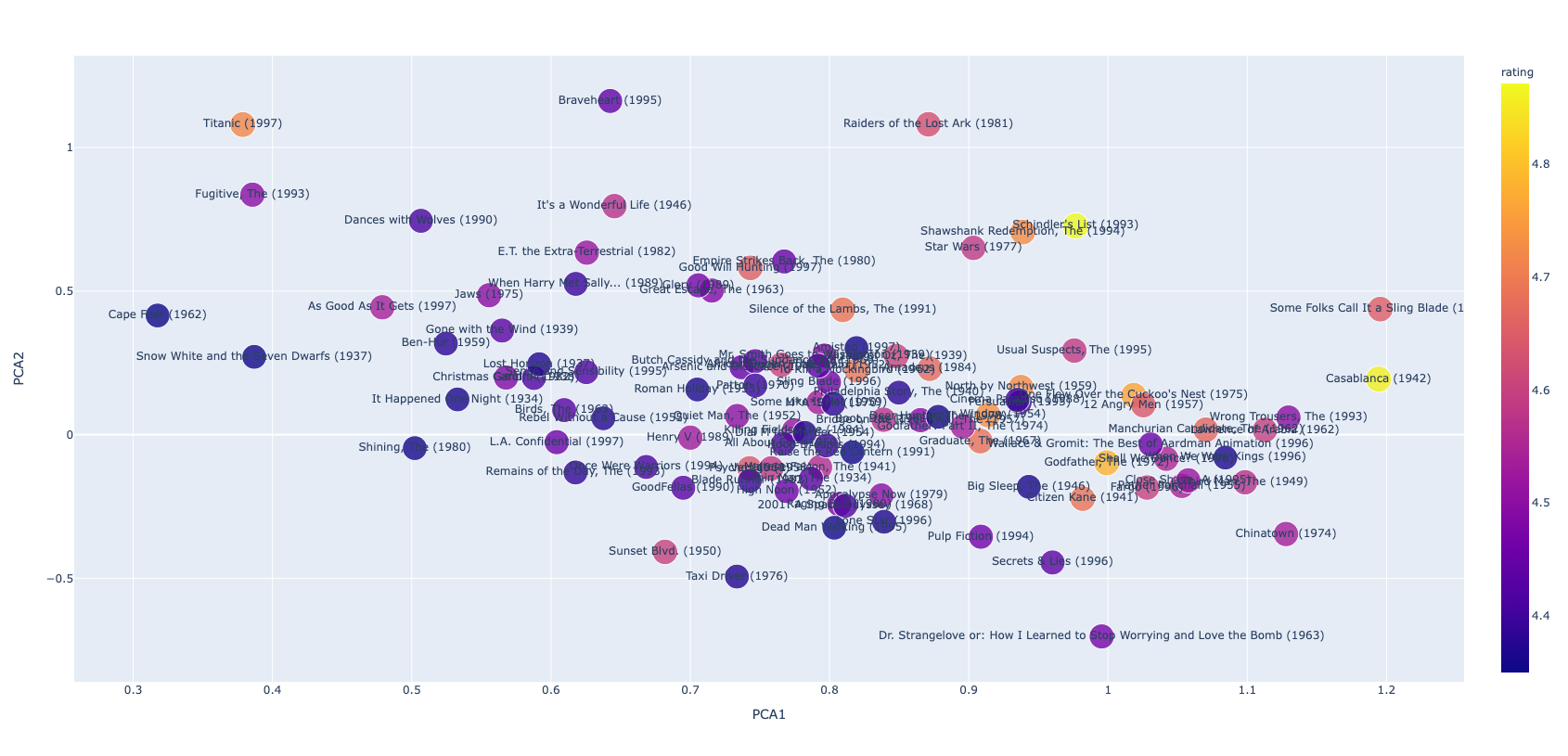
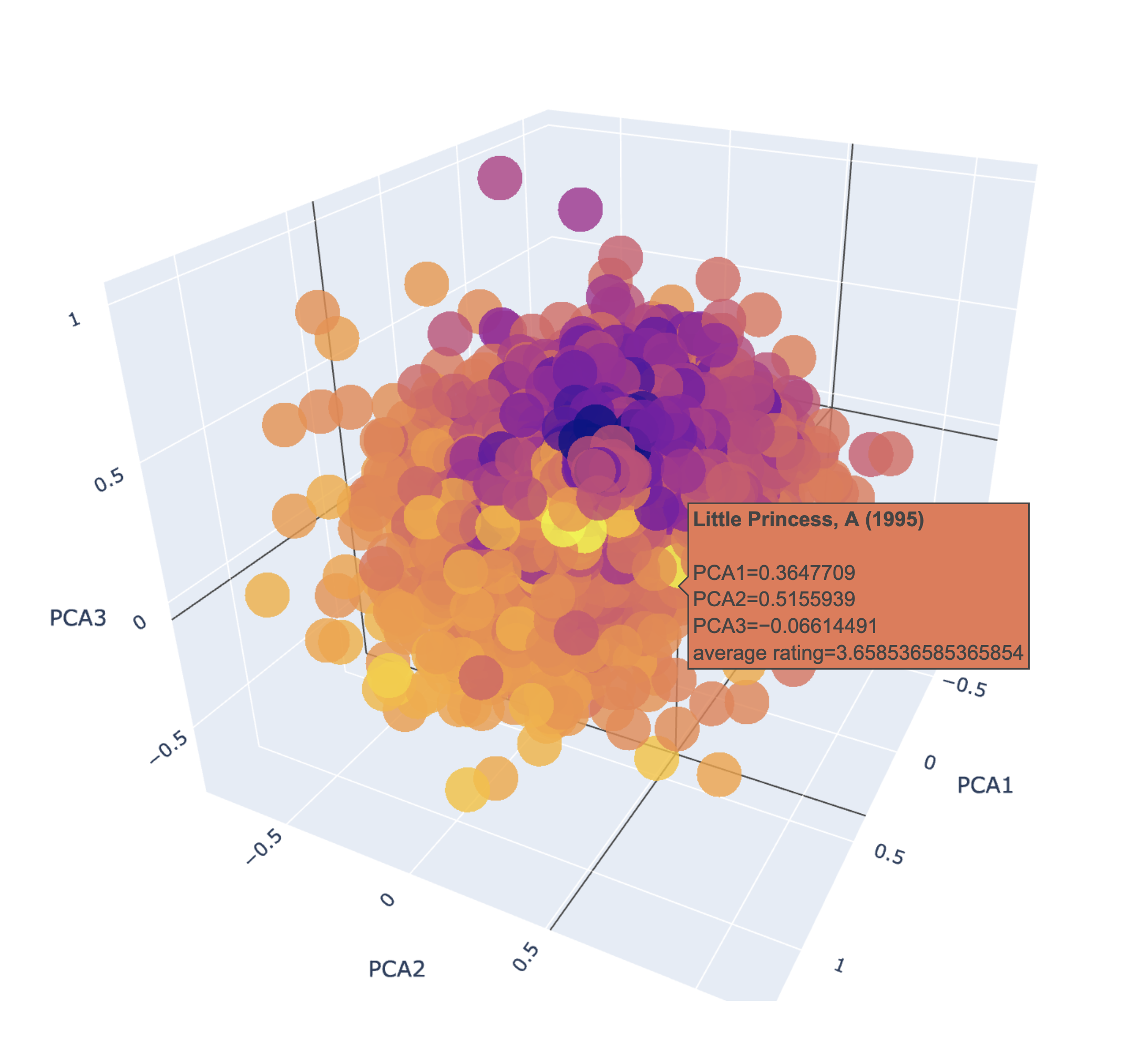
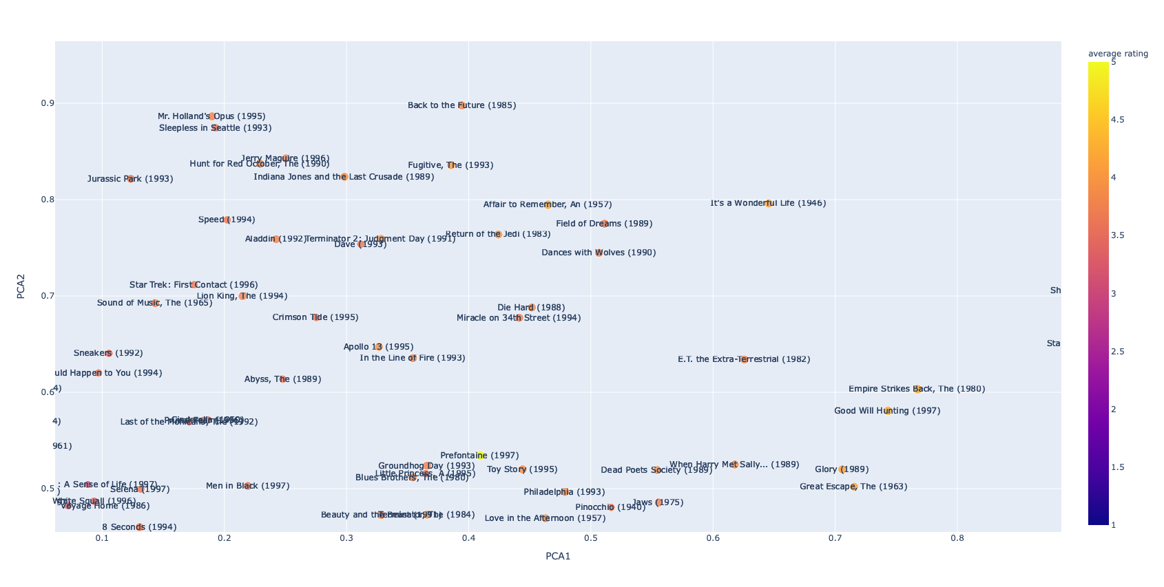
アイテム（映画）を2次元に可視化する関数 show_item_map

show_item_map

 show_item_map (learn, movies_df)

show_item_map関数の使用例

# fig, movies = show_item_map(learn, movies_df)
# plotly.offline.plot(fig);
# movies.head()

	movie	title	average rating	PCA1	PCA2	PCA3
0	1	Toy Story (1995)	3.878319	0.444091	0.520046	-0.033139
1	2	GoldenEye (1995)	3.206107	-0.039345	0.377593	0.204351
2	3	Four Rooms (1995)	3.033333	-0.270448	0.101434	0.574822
3	4	Get Shorty (1995)	3.550239	0.457936	0.075438	0.199581
4	5	Copycat (1995)	3.302326	-0.138418	0.573008	-0.084740

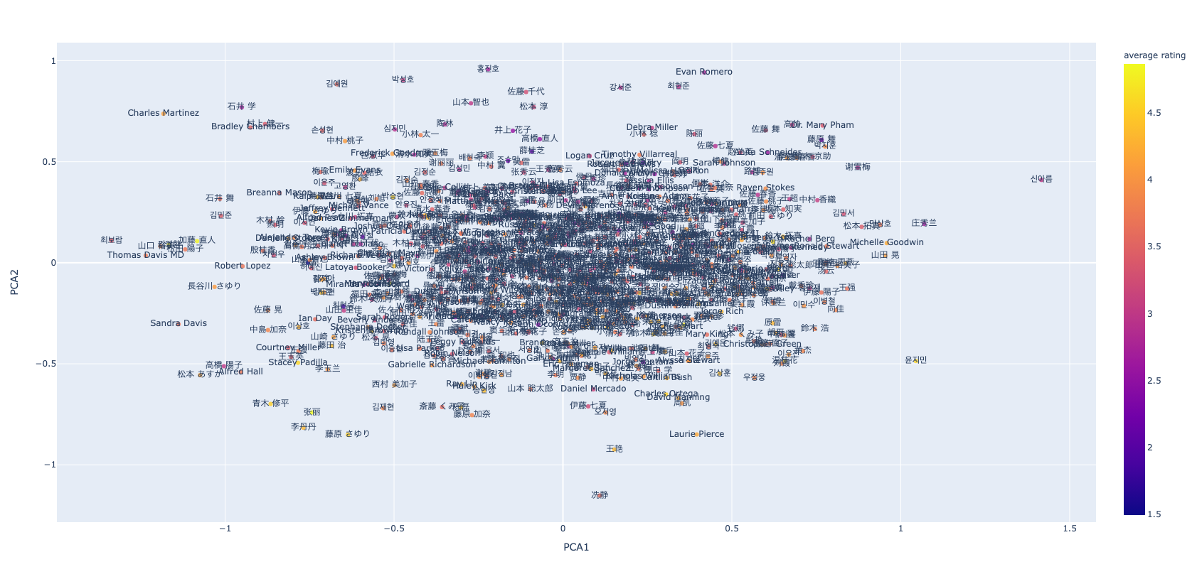
ユーザーを2次元に可視化する関数 show_user_map

show_user_map

 show_user_map (learn, users_df)

show_user_map関数の使用例

# fig, users = show_user_map(learn, users_df)
# plotly.offline.plot(fig);
# users.head()

	id	name	average rating	PCA1	PCA2	PCA3
0	1	Ryan Gallagher	3.610294	0.540301	-0.043214	-0.551639
1	2	박영길	3.709677	0.215085	-0.478103	-0.068856
2	3	後藤あすか	2.796296	0.225072	0.370120	-0.026158
3	4	Russell Reynolds	4.333333	-0.085290	0.185153	-0.412719
4	5	佐藤七夏	2.874286	0.451194	0.577116	-0.321961

ユーザーへの推奨アイテムを可視化する関数 show_recommend

show_recommend

 show_recommend (learn, movies_df, recommend_df, best=100)

# fig = show_recommend(learn, movies_df, recommend_df, best=100)
# plotly.offline.plot(fig);