mean = 100.
sigma = 10.
normal = norm(mean,sigma) #需要量
price = 100.   #販売価格
purchase = 70. #仕入れ値
demand = normal.rvs(100)
lostsales = 0.
salvage = 10. #バイトに半値で売るとき 50 :-)
loyality = 0.5
Q = 100 #発注量
QLB = 50
QUB = 130

retail_profit, seven_profit = [], []
for Q in range(QLB,QUB):

    profit_retail, profit_seven, lostsales_cost, salvage_value = 0,0,0,0
    for d in list(demand):
        purchase_cost = purchase*Q
        profit = price*min(Q,d)
        net_margin = profit-purchase_cost  #粗利益(通常会計 -> 本社利益と小売店利益は同じ)
        profit_retail +=  (net_margin + salvage*max(Q-d,0) -lostsales*max(d-Q,0))*(1.-loyality) #loyality = phi (=supplierへの利益分配率))
        profit_seven  += (net_margin+ salvage*max(Q-d,0)- lostsales*max(d-Q,0) )*loyality
        lostsales_cost += lostsales*max(d-Q,0) #機会損出費用
        salvage_value += salvage*max(Q-d,0)    #売れ残り価値

    retail_profit.append( profit_retail)
    seven_profit.append( profit_seven)

#print(profit_retail, profit_seven, lostsales_cost, salvage_cost)

#最適な発注量を求める => プロット
# min_cost = np.max
retail_profit2, seven_profit2 = [], []
for Q in range(QLB,QUB):

    profit_retail, profit_seven, lostsales_cost, salvage_value = 0,0,0,0
    for d in list(demand):
        purchase_cost = purchase*min(Q,d) #売れた分だけ仕入れ値を払う(コンビニ会計)
        profit = price*min(Q,d)
        net_margin = profit-purchase_cost #粗利益(コンビニ会計だとnet_marginが大きくなる)
        profit_retail += net_margin*(1.-loyality) -purchase*max(Q-d,0)+salvage*max(Q-d,0) -lostsales*max(d-Q,0)*(1.-loyality) #売れ残りに対する原価を店舗利益から引く(コンビニ会計)
        profit_seven  += net_margin*loyality- lostsales*max(d-Q,0)*loyality
        lostsales_cost += lostsales*max(d-Q,0) #機会損出費用
        salvage_value += salvage*max(Q-d,0)    #売れ残り価値

    retail_profit2.append( profit_retail)
    seven_profit2.append( profit_seven)

#print(profit_retail, profit_seven, lostsales_cost, salvage_cost)例題集:在庫最適化
在庫最適化の例題
cost_df = pd.DataFrame({"発注量":list(range(QLB,QUB)),"小売利益":retail_profit, "本社利益":seven_profit,
                       "小売利益(コンビニ会計)":retail_profit2, "本社利益(コンビニ会計)":seven_profit2})
cost_df.head()| 発注量 | 小売利益 | 本社利益 | 小売利益(コンビニ会計) | 本社利益(コンビニ会計) | |
|---|---|---|---|---|---|
| 0 | 50 | 50000.0 | 50000.0 | 50000.0 | 50000.0 |
| 1 | 51 | 51000.0 | 51000.0 | 51000.0 | 51000.0 |
| 2 | 52 | 52000.0 | 52000.0 | 52000.0 | 52000.0 |
| 3 | 53 | 53000.0 | 53000.0 | 53000.0 | 53000.0 |
| 4 | 54 | 54000.0 | 54000.0 | 54000.0 | 54000.0 |
fig = px.scatter(cost_df, x="発注量",y=["小売利益", "本社利益","小売利益(コンビニ会計)", "本社利益(コンビニ会計)" ])
plotly.offline.plot(fig);
#hide ## 生産計画モデル
最終工程の充填工程と前工程は独立に解ける.(中間の保管場所が制約にならないため.)
26の製品(最小と最大ロットサイズ);製造名称が親製品に対応?
25の充填ライン
データに需要がない. 人数制約がない.
集合
- 製品の集合 \(P\)
- 期の集合 \(T\)
- ラインの集合 \(L\)
パラメータ
- 需要量 \(d_{pt}\)
- 段取り費用 \(F_{pl}\)
- 生産費用 \(c_{pl}\)
- 在庫費用 \(h_p\)
- 最小,最大ロットサイズ \(MinL_{p}, MaxL_{p}\)
- 最大人数 \(MaxW_{t}\)
- 最大生産時間 \(UB_{lt}\)
- 必要人数 \(a_{pl}\)
- 生産時間 \(w_{pl}\)
- 段取り時間 \(SUT_{pl}\)
変数 - \(t\) 期の製造量 \(x_{plt}\) (整数) - \(t\) 期に段取りするとき \(1\) \(y_{plt}\) - \(t\) 期の在庫量 \(I_{pt}\)
\[ minimize \sum h_{p} I_{pt} + \sum F_{pl} y_{plt} + \sum c_{pl} x_{plt} \]
\[ I_{p,t-1} + \sum_{l} x_{plt} = d_{pt} + I_{pt} \ \ \ \forall p,t \]
\[ MinL_{p} y_{plt} \leq x_{plt} \leq MaxL_{p} y_{plt} \ \ \ \forall p,l, t \]
\[ \sum_{p} w_{pl} x_{plt} + SUT_{pl} y_{plt} \leq UB_{lt} \ \ \ \forall l, t \]
\[ \sum_{p,l} a_{pl} x_{plt} \leq MaxW_{t} \ \ \ \forall t \]
予測と在庫管理の融合
従来の需要予測の研究と在庫管理の研究は別々に行われてきた. 予測では,非定常な需要を仮定し,在庫管理では定常な分布を仮定する場合が多い. これらの2つの(おそらくサプライ・チェインに対して最も重要かつ最も多くの研究が行われてきた)モデルを構築することは,永年の研究者たちの夢であったが,いまだに実務的で納得するものは出ていない.
従来の研究の多くは,以下の2つに分類される.
- 綺麗な解析ができるような(実務的にはかなり特殊な)仮定の元での理論研究
- 実際の問題をなんとか解決するための(理論的な背景はほとんど考慮されていない)ヒューリスティクス
以下では,理論的にもある程度きちんとした枠組みで,かつ実際問題を解決可能な方法について考える.方針は以下の通り.
予測を行い誤差の分布を適当な分布で近似する.
リード時間分の予測需要の合計と分布に基づく安全在庫の和が変動型の基在庫レベルになる.
需要が負にならないようにスライドして,基在庫レベル最適化を行い,安全在庫量の最適化を行う.
安全在庫と需要予測に基づく確定在庫を合わせることによって,動的な基在庫レベルを導く.
Integrating Forecasting and Inventory Management
Traditional research on demand forecasting and inventory management have been conducted separately. Forecasting often assumes a non-stationary demand, while inventory management assumes a stationary distribution. Building these two (probably the most important and most studied) models for the supply chain has been a dream of researchers for a long time, but nothing practical and convincing has been produced yet.
Most conventional research can be divided into two categories.
- Theoretical research based on assumptions that allow for clean analysis (which are quite specific from a practical standpoint)
- Heuristics to somehow solve real problems (with little or no consideration of theoretical background).
In the following, we will consider methods that are both theoretically sound and capable of solving practical problems. The policy is as follows.
Make a forecast and approximate the distribution of the error with a suitable distribution.
The sum of the total demand forecast for the lead time and the safety stock based on the distribution is the base stock level for the variable type.
The base inventory level is optimized by sliding the demand so that it does not become negative, and the amount of safety stock is optimized.
The dynamic base stock level is derived by combining the safety stock and the fixed stock based on the demand forecast.
サンプル需要データの読み込み
プロモーションデータを付加した需要データを読み込む.顧客と製品を選択肢,1日単位の需要系列を生成する. 2019年の年初から2020年の年末までのデータであり,2020年10月以降を検証用として用いる.
予測手法は自動機械学習を用いる.この部分は深層学習やベイズ推論に置き換えても良い.
Loading sample demand data
Load the demand data with promotion data added. Choose customers and products, and generate a daily demand series. The data covers the period from the beginning of 2019 to the end of 2020, and the data after October 2020 is used for validation.
The forecasting method is based on automatic machine learning. This part can be replaced by deep learning or Bayesian inference.
promo_df = pd.read_csv(folder+"promo.csv", index_col=0)
demand_df = pd.read_csv(folder+"demand_with_promo_all.csv")
c = "仙台市"
p = "C"
print(c,p)
agg_period ="1d"
df, future = make_forecast_df(demand_df, customer=c, product=p,promo_df= promo_df, agg_period="1d", forecast_periods = 10)
horizon="2020/10/01"
best, result_df = automl(df, horizon, 5)| Model | MAE | MSE | RMSE | R2 | RMSLE | MAPE | TT (Sec) | |
|---|---|---|---|---|---|---|---|---|
| et | Extra Trees Regressor | 0.8184 | 1.4329 | 1.1970 | 0.9259 | 0.3454 | 0.3228 | 0.1400 |
| catboost | CatBoost Regressor | 0.9641 | 1.6140 | 1.2704 | 0.9166 | 0.4705 | 0.3642 | 1.2500 |
| rf | Random Forest Regressor | 0.9471 | 1.8677 | 1.3666 | 0.9035 | 0.3581 | 0.2946 | 0.1700 |
| lightgbm | Light Gradient Boosting Machine | 1.0635 | 2.0255 | 1.4232 | 0.8953 | 0.4909 | 0.3828 | 0.1600 |
| xgboost | Extreme Gradient Boosting | 1.0059 | 2.0651 | 1.4370 | 0.8933 | 0.4459 | 0.3132 | 0.3900 |
| gbr | Gradient Boosting Regressor | 1.1372 | 2.7493 | 1.6581 | 0.8579 | 0.4964 | 0.4625 | 0.0800 |
| dt | Decision Tree Regressor | 1.3407 | 5.5824 | 2.3627 | 0.7114 | 0.7269 | 0.5754 | 0.0100 |
| ada | AdaBoost Regressor | 2.3201 | 7.0186 | 2.6493 | 0.6372 | 0.9424 | 0.5857 | 0.0700 |
| ridge | Ridge Regression | 2.1316 | 7.4200 | 2.7240 | 0.6164 | 0.9256 | 0.9212 | 0.0000 |
| br | Bayesian Ridge | 2.1351 | 7.4732 | 2.7337 | 0.6137 | 0.9270 | 0.9264 | 0.0100 |
| lar | Least Angle Regression | 3.7772 | 18.6936 | 4.3236 | 0.0337 | 1.1358 | 1.2991 | 0.0100 |
| huber | Huber Regressor | 3.0573 | 19.5931 | 4.4264 | -0.0128 | 0.8909 | 0.6111 | 0.0200 |
| en | Elastic Net | 4.0496 | 19.6190 | 4.4293 | -0.0142 | 1.2366 | 1.1734 | 0.0000 |
| par | Passive Aggressive Regressor | 3.8849 | 19.8872 | 4.4595 | -0.0280 | 1.1862 | 1.0219 | 0.0000 |
| lr | Linear Regression | 4.1256 | 20.4303 | 4.5200 | -0.0561 | 1.2505 | 1.2217 | 0.0000 |
| lasso | Lasso Regression | 4.1243 | 20.4572 | 4.5230 | -0.0575 | 1.2509 | 1.2182 | 0.0000 |
| llar | Lasso Least Angle Regression | 4.7760 | 26.0867 | 5.1075 | -0.3485 | 1.3798 | 1.5266 | 0.0000 |
| omp | Orthogonal Matching Pursuit | 4.1709 | 28.0720 | 5.2983 | -0.4511 | 1.2779 | 1.0241 | 0.0000 |
| knn | K Neighbors Regressor | 7.1319 | 62.3846 | 7.8984 | -2.2248 | 1.7197 | 2.7013 | 0.0000 |
fig, error, result = predict_using_automl(df, future, best[0])
#plotly.offline.plot(fig);| Model | MAE | MSE | RMSE | R2 | RMSLE | MAPE | |
|---|---|---|---|---|---|---|---|
| 0 | Extra Trees Regressor | 0.8184 | 1.4329 | 1.1970 | 0.9259 | 0.3454 | 0.3228 |
検証用データに対する誤差分布の解析
検証用データ期間に対して1日単位の誤差を求め,最も適合する連続分布を求める.
リード時間内の誤差の和の分布を求め,同様に最も適合する連続分布を求める.
train_idx, valid_idx = prepare_index(df, horizon)
print(len(valid_idx))90error = result[:len(df)].Label - df.demand
error[valid_idx].hist(density=True);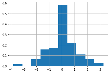
error[valid_idx]640 -0.88
641 -1.10
642 -0.18
643 0.47
644 -0.52
...
725 0.02
726 0.01
727 -0.85
728 0.05
729 0.06
Length: 90, dtype: float64#1日分の需要量(誤差)分布を求める
fig, best_dist, best_fit_name, best_fit_params = best_distribution(error[valid_idx])
#plotly.offline.plot(fig);
print(best_fit_name, best_fit_params)dgamma (0.5146404593477012, 0.019999999999999997, 1.4358365014276395)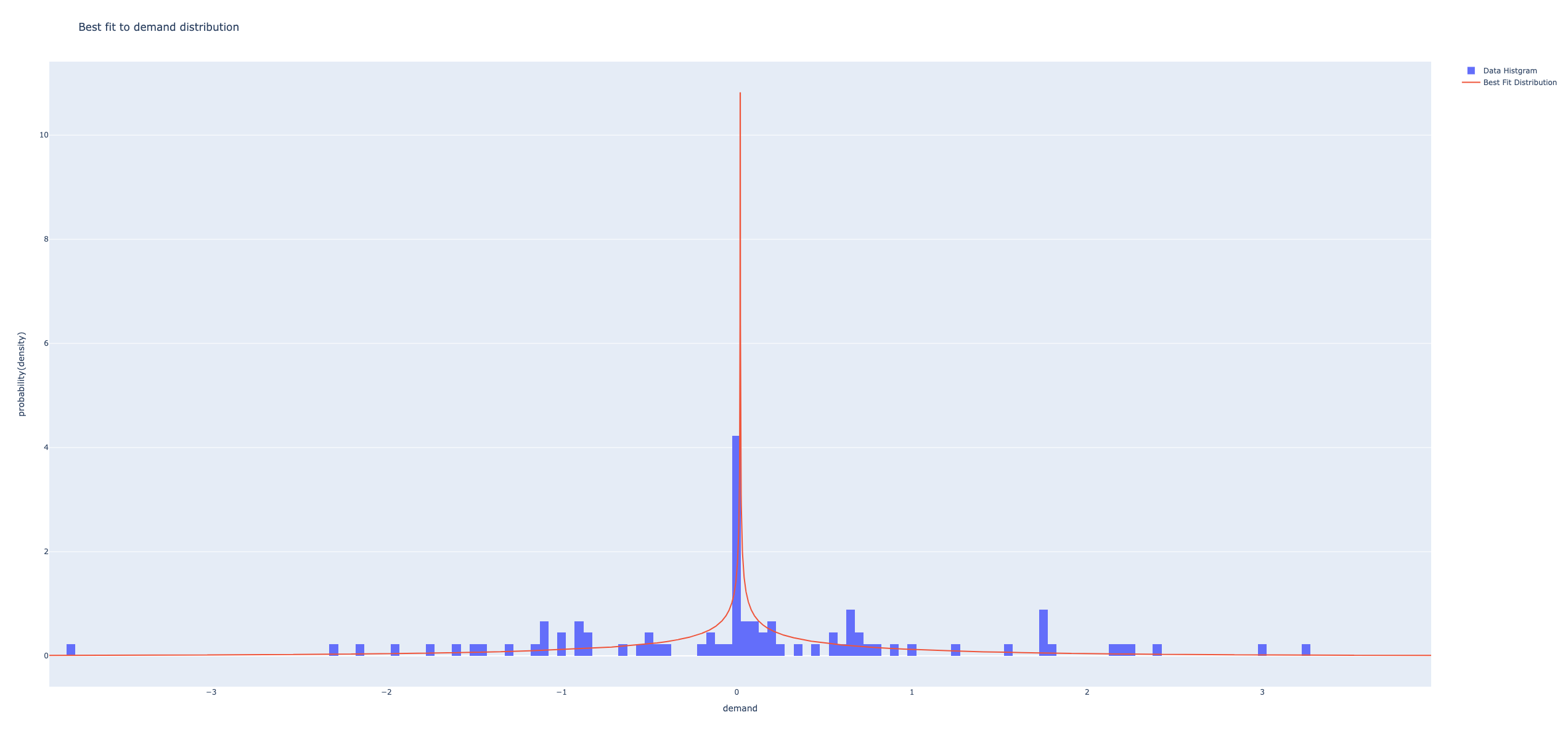
d = best_dist.rvs((5,10000))
pd.Series(d.sum(axis=0)).hist(density=True);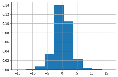
n = norm(loc=best_dist.mean()*5,scale=best_dist.std()*np.sqrt(5))
d2 = best_dist.rvs(10000)
pd.Series(d2).hist(density=True);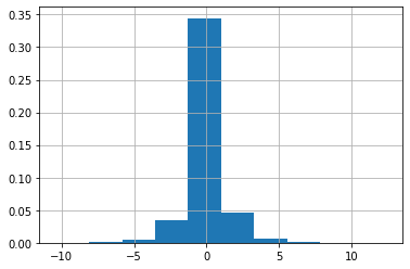
#正味補充(リード)時間内の最大在庫量を計算
Lmax = 50
MaxDemand = [0.]
for L in range(1,min(Lmax,len(data))): #リード時間
    df_error = pd.Series(error[valid_idx])
    data = df_error.rolling(window=L).sum()[L-1:].values #L日前から直前までの需要の合計
    fig, hist  = best_histogram(data)
    #plotly.offline.plot(fig2);
    MaxDemand.append( hist.ppf(0.95) )
#非減少にする
MaxDemand2 = []
max_ = MaxDemand[0]
for d in MaxDemand:
max_ = max(max_, d)
if d < max_:
MaxDemand2.append(max_)
else:
MaxDemand2.append(d)
pd.Series(MaxDemand2).plot();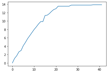
L = 5#リード時間
df_error = pd.Series(error[valid_idx])
data = df_error.rolling(window=L).sum()[L-1:].values #L日前から直前までの需要の合計
pd.Series(data).hist();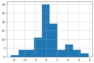
fig2, best_dist2, best_fit_name2, best_fit_params2  = best_distribution(data)
plotly.offline.plot(fig2);
print(best_fit_name2, best_fit_params2)
dgamma (0.7658916979282773, 0.10999999999999988, 1.766101465922829)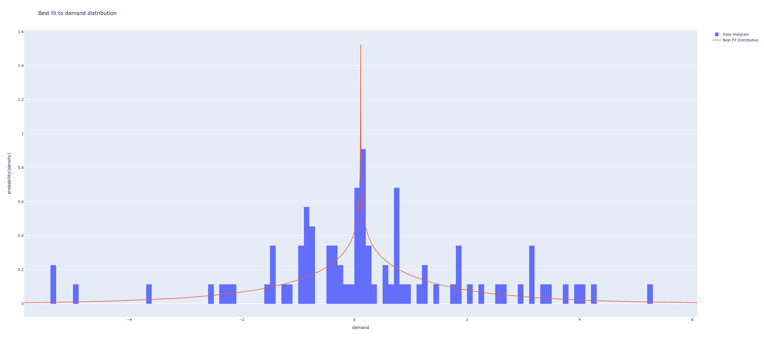
基在庫レベルの設定
誤差分布から定常な需要分布を生成する.
リード時間内の誤差分布から,初期基在庫レベルを以下の式で生成する.
品切れ費用 \(b\),在庫費用から臨界率を計算する.
\[ \omega = b/(b+h) \]
リード時間内の需要分布に対して,品切れ率が臨界率に一致するように安全在庫量を求める.
また,需要が負にならないように,それ以下になる確率が1%の値を \(0\) と設定することによって,需要を定数だけ大きくする. 毎日,この定数分だけの需要が発生すると仮定して,需要データを生成する.
この需要系列を利用して,定常状態の最適な基在庫レベルをシミュレーションに基づく最適化で行う.
n_samples = 10
n_periods = 1000
capacity = 10.
convergence = 1e-5
b = 100
h = 1
LT = L
critical_ratio = b/(b+h)
S = best_dist2.ppf(critical_ratio)
lb = best_dist.ppf(0.01)
print(S, lb )
demand = best_dist.rvs((n_samples,n_periods)) - lb #需要を分布が0以上になるようにシフトさせる.
S = S - lb*LT #基在庫レベルはリード時間内の定常需要だけ大きくする.
print(S)
6.106113612640433 -3.923975750210528
17.87804086327202n_samples = 10
n_periods = 1000
capacity = 1000.
convergence = 1e-5
b = 100
h = 1
LT = L
critical_ratio = b/(b+h)
S = best_dist2.ppf(critical_ratio)
lb = best_dist.ppf(0.01)
print(S, lb )
demand = best_dist.rvs((n_samples,n_periods)) - lb #需要を分布が0以上になるようにシフトさせる.
S = S - lb*LT #基在庫レベルはリード時間内の定常需要だけ大きくする.
print(S)
print("t: S dS Cost")
for iter_ in range(100):
dC, cost, I = base_stock_simulation(n_samples, n_periods, demand, capacity, LT, b, h, S)
S = S - .1*dC
print(f"{iter_}: {S:.2f} {dC:.3f} {cost:.2f}")
if dC**2<=convergence:
break6.106113612640433 -3.923975750210528
17.87804086327202
t: S dS Cost
0: 17.87 0.091 7.54
1: 17.86 0.081 7.54
2: 17.85 0.071 7.54
3: 17.85 0.071 7.54
4: 17.84 0.071 7.54
5: 17.83 0.061 7.54
6: 17.83 0.061 7.54
7: 17.82 0.061 7.54
8: 17.82 0.061 7.54
9: 17.81 0.051 7.54
10: 17.81 0.051 7.54
11: 17.80 0.051 7.54
12: 17.80 0.030 7.54
13: 17.79 0.030 7.54
14: 17.79 0.010 7.54
15: 17.79 0.010 7.54
16: 17.79 0.010 7.54
17: 17.79 0.010 7.54
18: 17.79 0.010 7.54
19: 17.79 0.010 7.54
20: 17.79 0.010 7.54
21: 17.79 0.010 7.54
22: 17.78 0.010 7.54
23: 17.78 0.010 7.54
24: 17.78 0.010 7.53
25: 17.78 0.010 7.53
26: 17.78 0.010 7.53
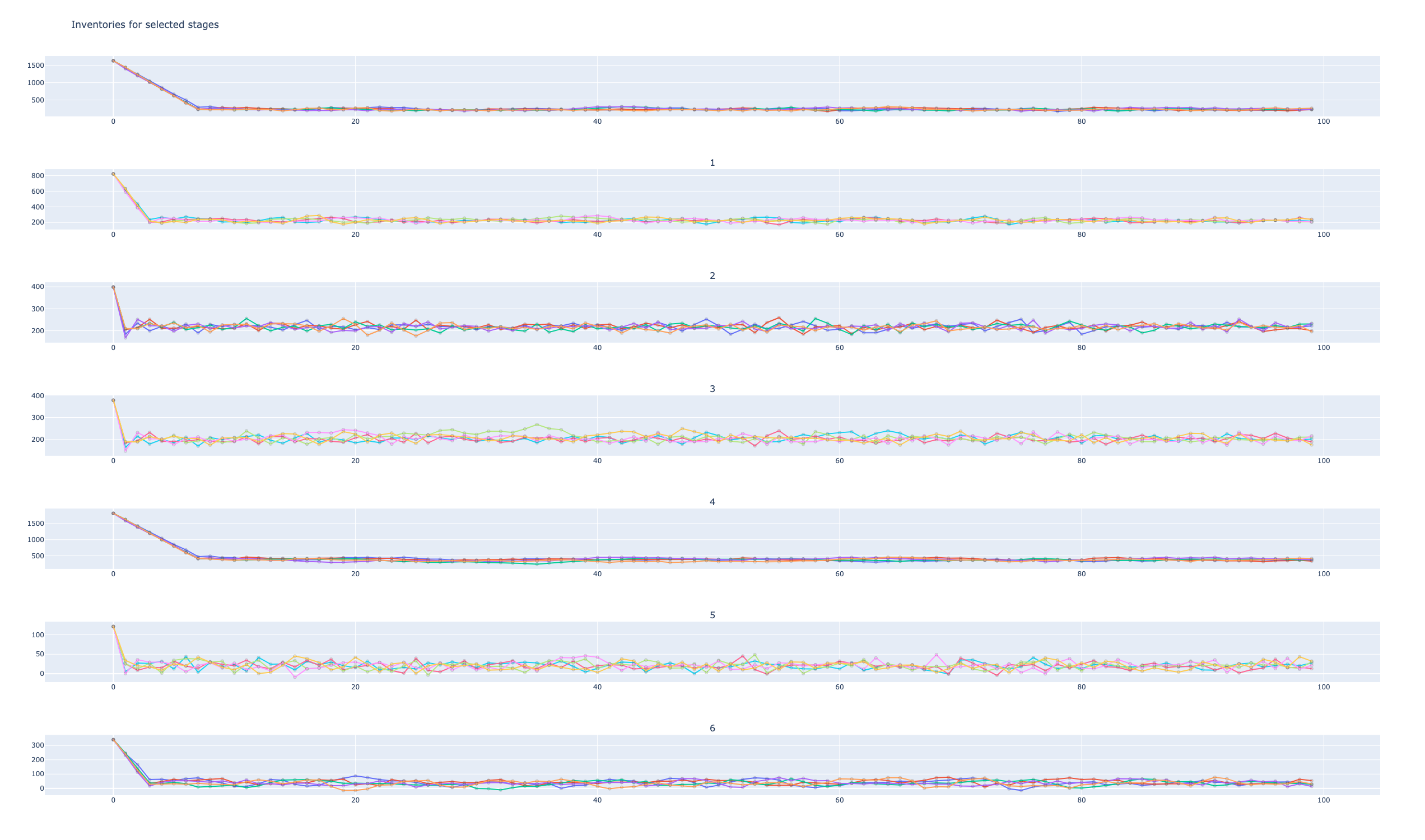
27: 17.78 0.000 7.53pd.DataFrame(I[0]).plot(); #在庫の推移の可視化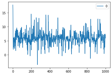
動的基在庫レベルの計算
定数分だけシフトした需要分を減じることによって,予測の誤差に対応するための安全在庫料量を計算する.
予測値は確定的な値として計算されるので,リード時間分の確定値の和だけ在庫を保持する.これに安全在庫分を加えたものが動的な基在庫レベルになる.
日々の運用は,在庫ポジションをこの値になるように発注(生産)を行う.
#安全在庫量
safety = S + lb*LT
print(safety)6.008873612640432#未来の確定値の需要予測(リード時間分の累積値)
future = pd.Series(result[len(df):].Label)
data = future.rolling(window=L).sum()[L-1:].values #L日前から直前までの需要の合計
dataarray([13.55, 13.47, 10.12, 6.89, 14.99, 21.15, 20.65, 20.65])#動的基在庫レベル
data + safetyarray([19.55887361, 19.47887361, 16.12887361, 12.89887361, 20.99887361,
27.15887361, 26.65887361, 26.65887361])#検証データでシミュレーション
future = result.Label[valid_idx]
data = future.rolling(window=L).sum()[L-1:].values #L日前から直前までの需要の合計
DS = data + safety #dynamic base stock level
dem = df.demand[valid_idx]I = np.zeros( len(dem)+1 )
I[0] = DS[0] #エシェロン在庫ポジション
for t, d in enumerate(dem):
I[t+1] = I[t] - d
order = max(DS[t+1] -I[t+1],0)
I[t+1] = I[t+1] + order
#print(t,d,I[t+1])
if t>=len(DS)-2:
breakpd.Series(I[:-3]).plot();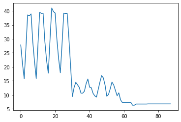
dem.plot();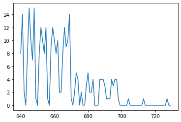
正規分布に近い需要関数の例
上の例ではzip分布に近い需要を仮定していた.以下では,正規分布に近い場合を考える.
demand_df = pd.read_csv(folder+"demand_normal.csv")
c = "仙台市"
p = "A"
print(c,p)
agg_period ="1d"
df, future = make_forecast_df(demand_df, customer=c, product=p,promo_df= None, agg_period="1d", forecast_periods = 0)
df.demand.max()
horizon="2019/10/01"
best, result_df = automl(df, horizon, 5)| Model | MAE | MSE | RMSE | R2 | RMSLE | MAPE | TT (Sec) | |
|---|---|---|---|---|---|---|---|---|
| lasso | Lasso Regression | 100.2628 | 15136.4229 | 123.0302 | 0.7174 | 0.0801 | 0.0656 | 0.0100 |
| ridge | Ridge Regression | 115.1678 | 21126.2422 | 145.3487 | 0.6056 | 0.0939 | 0.0716 | 0.0000 |
| llar | Lasso Least Angle Regression | 124.3677 | 22642.7084 | 150.4749 | 0.5773 | 0.1000 | 0.0847 | 0.0000 |
| lightgbm | Light Gradient Boosting Machine | 135.1054 | 26361.0052 | 162.3607 | 0.5079 | 0.1054 | 0.0912 | 0.0400 |
| omp | Orthogonal Matching Pursuit | 130.6787 | 27112.9591 | 164.6601 | 0.4938 | 0.1072 | 0.0880 | 0.0000 |
| gbr | Gradient Boosting Regressor | 140.5485 | 28375.8903 | 168.4514 | 0.4703 | 0.1097 | 0.0951 | 0.0400 |
| catboost | CatBoost Regressor | 151.5904 | 32636.8823 | 180.6568 | 0.3907 | 0.1175 | 0.1030 | 1.2700 |
| en | Elastic Net | 171.0394 | 42394.4023 | 205.8990 | 0.2086 | 0.1362 | 0.1163 | 0.0000 |
| et | Extra Trees Regressor | 177.6587 | 43153.4575 | 207.7341 | 0.1944 | 0.1327 | 0.1196 | 0.1400 |
| ada | AdaBoost Regressor | 185.1509 | 47749.3467 | 218.5162 | 0.1086 | 0.1402 | 0.1265 | 0.0500 |
| rf | Random Forest Regressor | 191.4697 | 51454.3014 | 226.8354 | 0.0394 | 0.1429 | 0.1296 | 0.1700 |
| xgboost | Extreme Gradient Boosting | 191.4150 | 53848.4531 | 232.0527 | -0.0053 | 0.1472 | 0.1308 | 0.3300 |
| par | Passive Aggressive Regressor | 191.9421 | 54763.1891 | 234.0154 | -0.0224 | 0.1515 | 0.1276 | 0.0000 |
| br | Bayesian Ridge | 195.9908 | 57561.6403 | 239.9201 | -0.0746 | 0.1564 | 0.1327 | 0.0000 |
| huber | Huber Regressor | 196.6167 | 58014.9136 | 240.8629 | -0.0831 | 0.1570 | 0.1332 | 0.0100 |
| lr | Linear Regression | 197.9349 | 58133.7969 | 241.1095 | -0.0853 | 0.1571 | 0.1340 | 0.0000 |
| lar | Least Angle Regression | 212.4354 | 61619.4643 | 248.2327 | -0.1503 | 0.1696 | 0.1315 | 0.0100 |
| dt | Decision Tree Regressor | 223.6154 | 71599.5055 | 267.5808 | -0.3367 | 0.1597 | 0.1475 | 0.0000 |
| knn | K Neighbors Regressor | 235.7868 | 79601.6484 | 282.1376 | -0.4861 | 0.1833 | 0.1647 | 0.0000 |
fig, error, result = predict_using_automl(df, future, best[0])
plotly.offline.plot(fig);| Model | MAE | MSE | RMSE | R2 | RMSLE | MAPE | |
|---|---|---|---|---|---|---|---|
| 0 | Lasso Regression | 100.2628 | 15136.4229 | 123.0302 | 0.7174 | 0.0801 | 0.0656 |
train_idx, valid_idx = prepare_index(df, horizon)
print(len(valid_idx))
error = result.Label - df.demand
error[valid_idx].hist(density=True);91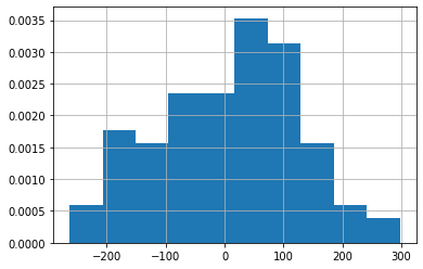
fig, best_dist, best_fit_name, best_fit_params = best_distribution(error[valid_idx])
plotly.offline.plot(fig);
print(best_fit_name, best_fit_params)mielke (2.6729912087197274, 11.291010366009026, -373.2172202339409, 503.0204118518145)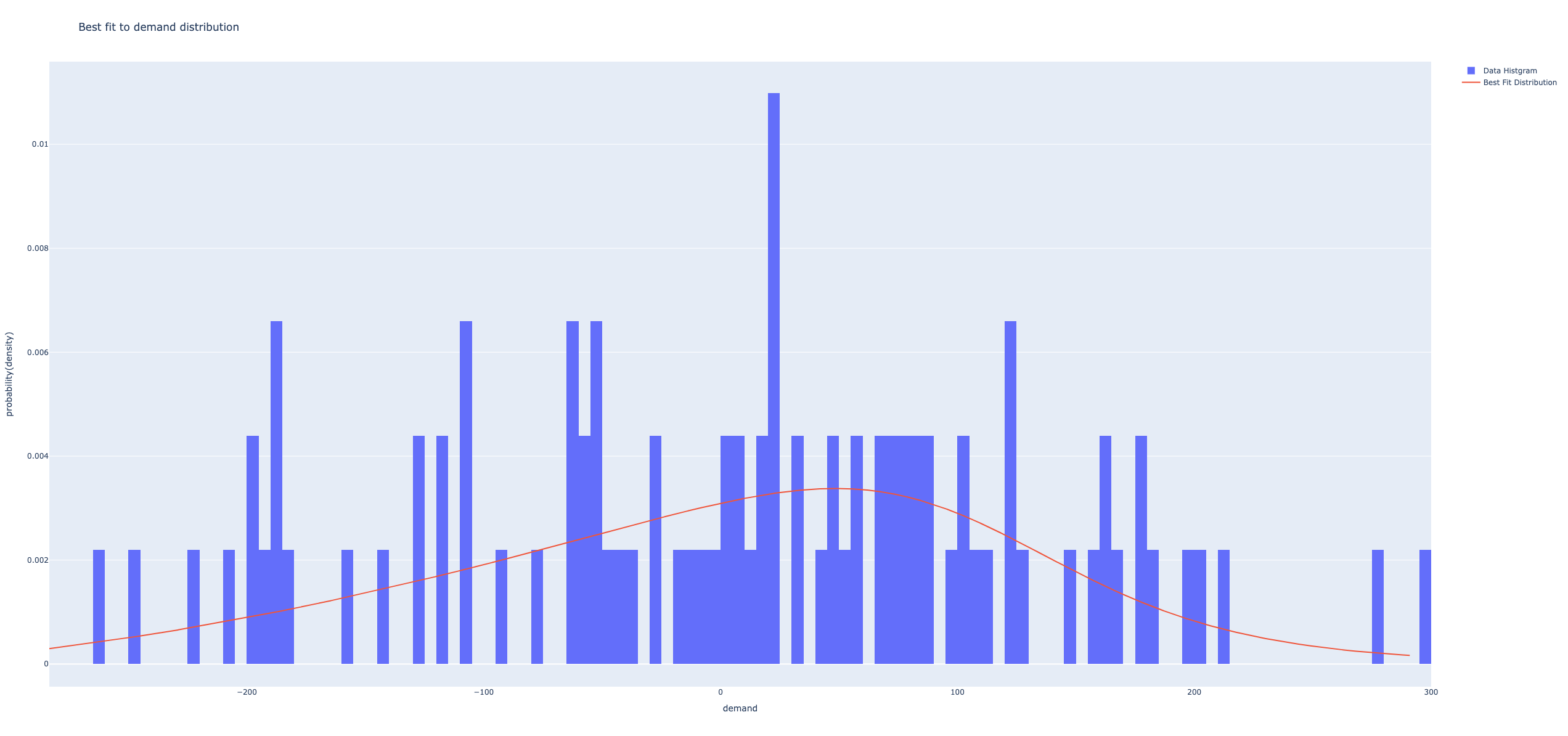
L = 3 #リード時間
df_error = pd.Series(error[valid_idx])
data = df_error.rolling(window=L).sum()[L-1:].values #L日前から直前までの需要の合計fig2, best_dist2, best_fit_name2, best_fit_params2 = best_distribution(data)
plotly.offline.plot(fig2);
print(best_fit_name2, best_fit_params2)gausshyper (0.5815996180621221, 3.799377992229532, -5.653814263450716, 2.624922751643501, -605.2475585937501, 1374.3047245376556)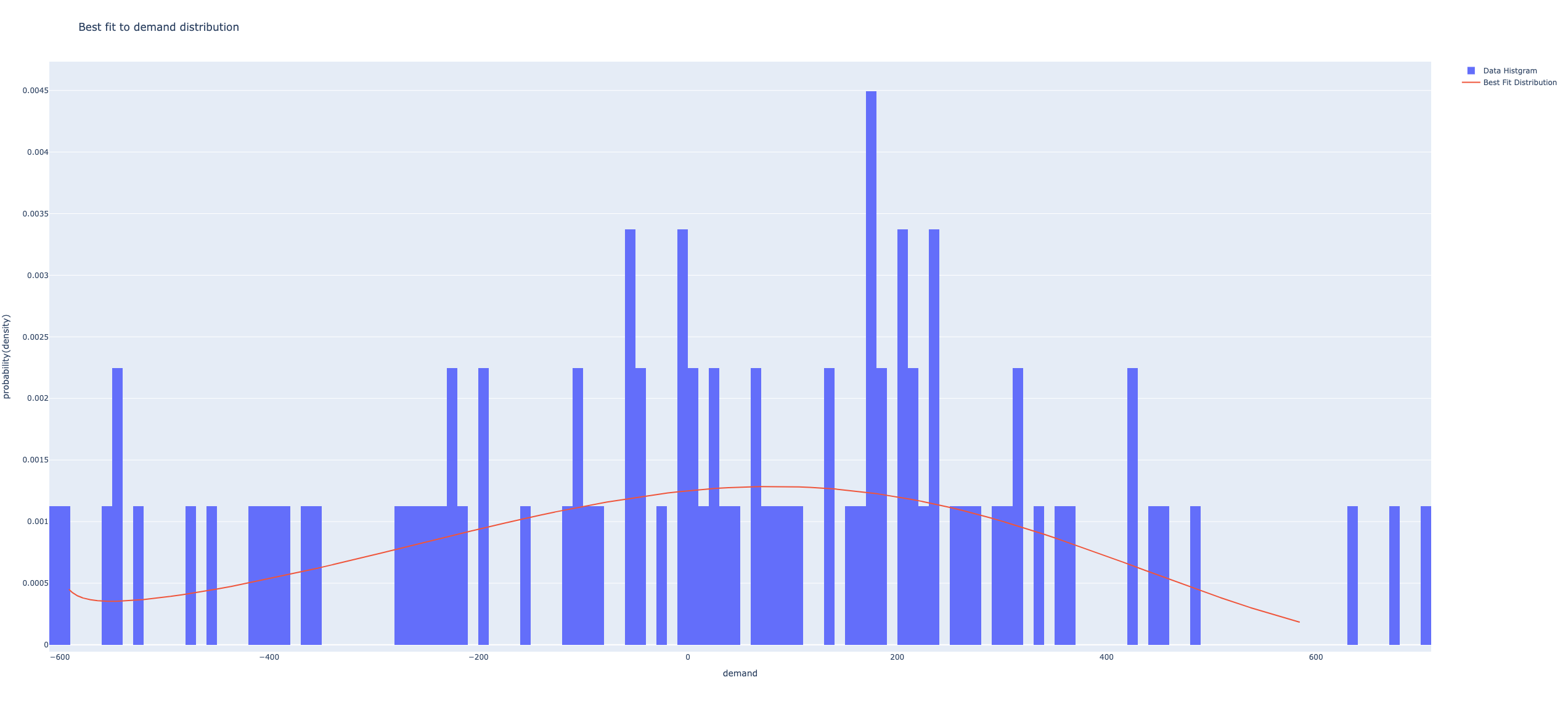
基在庫レベルの設定
n_samples = 10
n_periods = 1000
capacity = 1000.
convergence = 1e-5
b = 100
h = 1
LT = L
critical_ratio = b/(b+h)
S = best_dist2.ppf(critical_ratio)
lb = best_dist.ppf(0.01)
print(S, lb )
demand = best_dist.rvs((n_samples,n_periods)) - lb #需要を分布が0以上になるようにシフトさせる.
S = S - lb*LT #基在庫レベルはリード時間内の定常需要だけ大きくする.
print(S)
print("t: S dS Cost")
for iter_ in range(100):
dC, cost, I = base_stock_simulation(n_samples, n_periods, demand, capacity, LT, b, h, S)
S = S - 10.*dC
print(f"{iter_}: {S:.2f} {dC:.3f} {cost:.2f}")
if dC**2<=convergence:
break585.0727636548719 -283.39988265249485
1435.2724116123563
t: S dS Cost
0: 1428.10 0.717 580.84
1: 1421.03 0.707 575.75
2: 1413.96 0.707 570.74
3: 1407.49 0.646 566.01
4: 1401.53 0.596 562.02
5: 1395.67 0.586 558.49
6: 1390.22 0.545 555.13
7: 1385.27 0.495 552.26
8: 1381.03 0.424 549.95
9: 1377.49 0.354 548.29
10: 1374.26 0.323 547.06
11: 1371.13 0.313 546.03
12: 1368.40 0.273 545.12
13: 1365.77 0.263 544.37
14: 1363.24 0.253 543.70
15: 1360.92 0.232 543.10
16: 1358.90 0.202 542.59
17: 1357.18 0.172 542.21
18: 1355.56 0.162 541.92
19: 1354.05 0.152 541.67
20: 1352.73 0.131 541.46
21: 1351.42 0.131 541.29
22: 1350.41 0.101 541.13
23: 1349.70 0.071 541.05
24: 1348.99 0.071 541.00
25: 1348.29 0.071 540.95
26: 1347.88 0.041 540.91
27: 1347.48 0.041 540.89
28: 1347.17 0.030 540.88
29: 1346.87 0.030 540.87
30: 1346.66 0.020 540.86
31: 1346.46 0.020 540.85
32: 1346.26 0.020 540.85
33: 1346.16 0.010 540.85
34: 1346.05 0.010 540.85
35: 1345.95 0.010 540.84
36: 1345.85 0.010 540.84
37: 1345.75 0.010 540.84
38: 1345.65 0.010 540.84
39: 1345.54 0.010 540.84
40: 1345.44 0.010 540.84
41: 1345.34 0.010 540.84
42: 1345.24 0.010 540.84
43: 1345.14 0.010 540.84
44: 1345.14 0.000 540.83pd.DataFrame(I[0]).plot(); #在庫の推移の可視化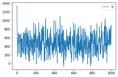
動的基在庫レベルの設定と検証データでシミュレーション
#安全在庫量
safety = S + lb*LT
print(safety)
#検証データでシミュレーション
future = result.Label[valid_idx]
data = future.rolling(window=L).sum()[L-1:].values #L日前から直前までの需要の合計
DS = data + safety #dynamic base stock level
dem = df.demand[valid_idx]
I = np.zeros( len(dem)+1 )
I[0] = DS[0] #エシェロン在庫ポジション
for t, d in enumerate(dem):
    I[t+1] = I[t] - d
    order = max(DS[t+1] -I[t+1],0)
    I[t+1] = I[t+1] + order
    #print(t,d,I[t+1])
    if t>=len(DS)-2:
        break
pd.Series(I[:-3]).plot();494.93576365487047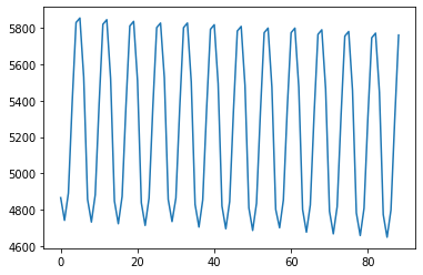
ネットワーク型の例
#7点の一般型ネットワークの例題
n = 7
G = SCMGraph()
for i in range(n):
    G.add_node(i)
G.add_edges_from([(0, 2), (1, 2), (2,4), (3,4), (4,5), (4,6)])

z = np.full(len(G),1.65)
h = np.array([1,1,3,1,5,6,6])
mu = np.array([200,200,200,200,200,100,100])
sigma = np.array([14.1,14.1,14.1,14.1,14.1,10,10])
LTUB = np.array([0,0,0,0,0,3,1], int)

ProcTime = np.array([6,2,3,3,3,3,3], int) # 動的最適化の例題と合わせるため、生産時間から保証リード時間上限を減じてある

best_cost, best_sol, best_NRT, best_MaxLI, best_MinLT  = tabu_search_for_SSA(G, ProcTime,  LTUB, z, mu, sigma, h, max_iter = 10, TLLB =1, TLUB =3, seed = 1)
print("最良値", best_cost)
print("最良解", best_sol)
print("正味補充時間", best_NRT)
print("最大補充リード時間", best_MaxLI)
print("最小保証リード時間", best_MinLT)

pos = G.layout()
stage_df, bom_df = make_df_for_SSA(G, pos, ProcTime, LTUB, z, mu, sigma, h, best_NRT, best_MaxLI, best_MinLT)
stage_df.to_csv(folder_bom + "stage_ex1.csv")
bom_df.to_csv(folder_bom + "bom_ex1.csv")

fig, G, pos = draw_graph_for_SSA_from_df(stage_df, bom_df)
#fig.show()
nx.draw(G, pos=pos)
最良値 514.8330943986502
最良解 [1 1 0 0 1 0 1]
正味補充時間 [6. 2. 0. 0. 6. 0. 2.]
最大補充リード時間 [6. 2. 3. 3. 6. 3. 3.]
最小保証リード時間 [0. 0. 3. 3. 0. 3. 1.]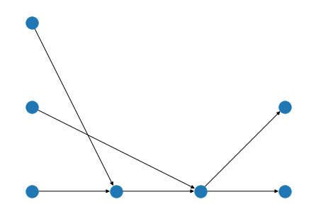
stage_df = pd.read_csv(folder_bom + "stage_ex1.csv")
bom_df = pd.read_csv(folder_bom + "bom_ex1.csv")
best_cost, stage_df, bom_df, fig = solve_SSA(stage_df, bom_df)
stage_df| Unnamed: 0 | name | net_replenishment_time | max_guaranteed_LT | processing_time | replenishment_LT | guaranteed_LT | z | average_demand | sigma | h | b | capacity | x | y | |
|---|---|---|---|---|---|---|---|---|---|---|---|---|---|---|---|
| 0 | 0 | 0 | 6.0 | 0 | 6 | 6.0 | 0.0 | 1.65 | 200 | 14.1 | 1 | 8.8 | 2000.0 | 0 | 0 |
| 1 | 1 | 1 | 2.0 | 0 | 2 | 2.0 | 0.0 | 1.65 | 200 | 14.1 | 1 | 8.8 | 2000.0 | 0 | 2 |
| 2 | 2 | 2 | 0.0 | 0 | 3 | 3.0 | 3.0 | 1.65 | 200 | 14.1 | 3 | 26.3 | 2000.0 | 1 | 0 |
| 3 | 3 | 3 | 0.0 | 0 | 3 | 3.0 | 3.0 | 1.65 | 200 | 14.1 | 1 | 8.8 | 2000.0 | 0 | 1 |
| 4 | 4 | 4 | 6.0 | 0 | 3 | 6.0 | 0.0 | 1.65 | 200 | 14.1 | 5 | 43.9 | 2000.0 | 2 | 0 |
| 5 | 5 | 5 | 0.0 | 3 | 3 | 3.0 | 3.0 | 1.65 | 100 | 10.0 | 6 | 52.7 | 1000.0 | 3 | 0 |
| 6 | 6 | 6 | 2.0 | 1 | 3 | 3.0 | 1.0 | 1.65 | 100 | 10.0 | 6 | 52.7 | 1000.0 | 3 | 1 |
cost, stage_df, I, cost_list, phi_list = periodic_inv_opt_fit_one_cycle(stage_df, bom_df, max_iter = 1000, n_samples = 10,
                                                                        n_periods = 100, seed = 1, lr_find=False, max_lr =6.0, moms=(0.85,0.95))
ELT= [21. 17. 13. 13. 11. 1. 3.]
S= [4306.61362354 3495.92405238 2683.88315042 2683.88315042 2277.16127575
116.5 328.57883832]
t: Cost |dC| S
0: 16082.26, 2384121.79078 [4306.61362354 3495.92405238 2683.88315042 2683.88315042 2277.16127575
116.5 328.57883832]
Best: 16054.62 [4294.07257219 3509.66262327 2667.975591 2687.85892252 2286.37514486
124.01255267 341.92807231]