import numpy as np
import matplotlib.pyplot as plt
from sortedcontainers import *
from timeit import default_timer as timer

import seaborn as sns; sns.set()  # for plot styling
from matplotlib.gridspec import GridSpec

def facility_location(clients, facilities, distances_list, c, opening_cost):
    """
        Implementation of algorithm outline found on page 183 of
        "The Design of Approximation Algorithms" by Williamson and Shmoys,
        and page 282 of "Approximation Algorithms for Metric Facility
        Location and k-Median Problems Using the Primal-Dual Schema and
        Lagrangian Relaxation" by Jain and Vazirani

        Takes as input a lists representing the facilites and clients,
        a (sorted) list of distances, and an integer for the facility opening cost.
        Executes the primal-dual uncapacitated facility location algorithm
        and finds a good approximate assignment for clients to facilities.
    """
    print("Starting primal-dual algorithm")

    start = timer()

    # Variable c_ij -- the distance between facility i and client j
    # Assume this is already in sorted order
    client_distances = distances_list
    num_client_distances = len(client_distances)

    # Variable w -- how much a client contributes to a particular facility
    # client_w[i][j] stores the time when client j starts to contribute to facility i
    client_w = [[-1 for j in range(len(clients))] for i in range(len(facilities))]

    # Record contribution when clients are declared connected
    client_v = [-1 for j in range(len(clients))]

    # We assume all facilitiy costs are equal
    facility_opening_cost = [opening_cost] * len(facilities)

    # Variable S -- gets a copy of the list of clients
    # Each client stores a list of facilities that it's assigned to
    # Coordinate 2 says if the client is currently open
    clients_copy = [[x, []] for x in clients]
    num_open_clients = len(clients_copy)

    # Variable T -- starts empty, but will accept facilities
    open_facilities = [-1] * len(facilities)

    # Initial time each facility will be paid for is one more than lambda
    # Second coordinate keeps track of the facility index

    maximum_distance_plus_one = opening_cost + 1
    facility_pay_schedule = [[maximum_distance_plus_one, x] for x in range(len(facilities))]
    next_paid_facility = SortedList(facility_pay_schedule)

    # Keep track of the index of the edge we service next
    current_edge_index = 0

    # Keep track of how much time has passed
    current_time = 0

    # Want to track how many times we update facility cost
    counter = [0]

    # Here we flag "closed" facilities with the value -1
    while num_open_clients > 0:

        if current_edge_index == num_client_distances:
            print("All edges have been evaluated. Continuing algorithm")
            # What if the algorithm needs more time?
            while not next_paid_facility == []:
                next_facility = next_paid_facility[0]
                if next_facility[0] >= 0:
                    current_time = next_facility[0]
                num_open_clients = update_facilities(next_facility[1], open_facilities[next_facility[1]][1], open_facilities, facility_pay_schedule, facility_opening_cost, next_paid_facility, clients_copy, num_open_clients, client_w, client_v, current_time)
                if num_open_clients <= 0:
                    break
            break

        distance = client_distances[current_edge_index]
        next_edge = distance[0]

        # Decide which event happens next
        if not next_paid_facility == []:
            next_facility = next_paid_facility[0]
        else:
            # Don't go here!
            next_facility = [next_edge + 1, 0]
        if next_edge <= next_facility[0]:
            # An edge goes tight
            # if not clients_copy[distance[2]] == -1:
            num_open_clients = service_tight_edge(open_facilities, facilities, clients_copy, distance, client_w, facility_opening_cost, facility_pay_schedule, next_paid_facility, num_open_clients, counter, client_v)
            current_time = distance[0]
            current_edge_index += 1
        else:
            # A facility is now paid for
            if next_facility[0] >= 0:
                current_time = next_facility[0]
            num_open_clients = update_facilities(next_facility[1], open_facilities[next_facility[1]][1], open_facilities, facility_pay_schedule, facility_opening_cost, next_paid_facility, clients_copy, num_open_clients, client_w, client_v, current_time)

    end = timer()
    print("Finished primal-dual algorithm. Time:", end - start)
    print("current_time:",current_time)

    # Some facilities might be paid for now, but haven't officially opened.
    # We fix that here.

    for i in range(len(facilities)):
        if not facility_pay_schedule[i] == -1:
            # Update client contribution to facility i
            # Only update pay from clients that are not yet connected

            num_clients_facility_i = len(open_facilities[i][1])
            update_client_pay = num_clients_facility_i * (current_time - open_facilities[i][2])
            open_facilities[i][3] += update_client_pay
            current_client_pay = open_facilities[i][3]

            if current_client_pay >= facility_opening_cost[i]:
                # Clients connected to facility i are removed from contributing to other facilities
                num_open_clients = update_facilities(i, open_facilities[i][1], open_facilities, facility_pay_schedule, facility_opening_cost, next_paid_facility, clients_copy, num_open_clients, client_w, client_v, current_time)


    pruning_primal_obj, pruning_opened_facilities, extra_cost = cluster_assignment_via_pruning(clients, facilities, client_w, c, facility_pay_schedule, client_v, opening_cost)

    print("num open facilities:", len(pruning_opened_facilities))

    # plot_final_points(clients, client_assignments)
    for x in pruning_opened_facilities:
        x[0] = facilities[x[0]]

    plot_final_clusters(pruning_opened_facilities)

def service_tight_edge(open_facilities, facilities, clients_copy, distance, client_w, facility_opening_cost, facility_pay_schedule, next_paid_facility, num_open_clients, counter, client_v):
    """
        Subroutine for the facility location algorithm for the event that
        an edge i,j goes tight
    """

    i = distance[1]
    j = distance[2]
    # print("Checking connection", i, j, "at time", distance[0])

    # Set the time for when client j starts to contribute
    if not clients_copy[j] == -1:
        client_w[i][j] = distance[0]

    # check to see if client j neighbors facility i
    # Assign and remove it if it does, provided the facility is paid for
    if facility_pay_schedule[i] == -1:
        if not clients_copy[j] == -1:
            open_facilities[i][1].add(j)
        num_open_clients = update_facilities(i, [j], open_facilities, facility_pay_schedule, facility_opening_cost, next_paid_facility, clients_copy, num_open_clients, client_w, client_v, distance[0])

    # Otherwise, client j contributes to the cost of facility i
    # Update contributions of other clients too
    else:
        if not clients_copy[j] == -1:
            clients_copy[j][1] += [i]
        # If facility i currently has no contributing clients
        if open_facilities[i] == -1:
            # Second coordinate -- track clients contributing to facility i
            # Third coordinate tracks times of last cost update
            # Fourth coordinate tracks running contribution of clients so far
            open_facilities[i] = [facilities[i], SortedList(), distance[0], 0]
            open_facilities[i][1].add(j)
            # Update when facility i will be paid for.
            next_paid_facility.remove([facility_pay_schedule[i][0], i])
            facility_pay_schedule[i][0] = facility_opening_cost[i]
            next_paid_facility.add([facility_pay_schedule[i][0], i])

        # Facility i already has some clients
        else:
            # Update client contribution to facility i
            num_clients_facility_i = len(open_facilities[i][1])

            update_client_pay = num_clients_facility_i * (distance[0] - open_facilities[i][2])
            open_facilities[i][3] += update_client_pay
            # open_facilities[i][3] += new_client_pay
            current_client_pay = open_facilities[i][3]
            # print("Facility",i,"now will be paid in",facility_pay_schedule[i][0] - current_client_pay)

            # Add client j to facility i
            if not clients_copy[j] == -1:
                open_facilities[i][1].add(j)
            open_facilities[i][2] = distance[0]

            if current_client_pay >= facility_opening_cost[i]:
                # Clients connected to facility i are removed from contributing to other facilities
                num_open_clients = update_facilities(i, open_facilities[i][1], open_facilities, facility_pay_schedule, facility_opening_cost, next_paid_facility, clients_copy, num_open_clients, client_w, client_v, distance[0])

            else:
                # Update when facility i will be paid for
                counter[0] += 1

                next_paid_facility.remove([facility_pay_schedule[i][0], i])
                if not len(open_facilities[i][1]) == 0:
                    remaining_time = (facility_opening_cost[i] - current_client_pay) / len(open_facilities[i][1])
                else:
                    # No currently contributing clients, so it should not get paid for anytime soon
                    remaining_time = facility_opening_cost[i] - distance[0] + 1
                # print("new pay schedule is", facility_pay_schedule[i][0])
                facility_pay_schedule[i][0] = distance[0] + remaining_time
                next_paid_facility.add([facility_pay_schedule[i][0], i])

    return num_open_clients

def update_facilities(i, update_clients, open_facilities, facility_pay_schedule, facility_opening_cost, next_paid_facility, clients_copy, num_open_clients, client_w, client_v, current_time):
    """
        Facility i is now paid for, so we declare its clients to be connected to it.

        We only update clients specified in update_clients
    """
    # iterate over clients contributing to facility i
    clients_to_add = []
    for j in update_clients:
        if not clients_copy[j] == -1:
            # declare client j to be connected
            # print("Client",j,"connects to facility", i,"at time", current_time)

            # Remove client j from contributing to anymore facilities
            # Update when other facilities are going to be paid for
            for f in clients_copy[j][1]:
                if not open_facilities[f] == -1 and not f == i:

                    if not facility_pay_schedule[f] == -1:
                        if not client_w[f][j] == -1:
                            next_paid_facility.remove([facility_pay_schedule[f][0], f])
                            # print("Updating", f, "old val", facility_pay_schedule[f][0])
                            # Record and update contribution of client j to facility f
                            num_clients_facility_f = len(open_facilities[f][1])
                            update_client_pay = num_clients_facility_f * (current_time - open_facilities[f][2])
                            open_facilities[f][3] += update_client_pay
                            current_client_pay = open_facilities[f][3]
                            facility_pay_schedule[f][0] = facility_opening_cost[f] - current_client_pay
                            open_facilities[f][2] = current_time
                            if not len(open_facilities[f][1]) == 0:
                                if j in open_facilities[f][1]:
                                    if len(open_facilities[f][1]) > 1:
                                        remaining_time = (facility_opening_cost[f] - current_client_pay) / (len(open_facilities[f][1]) - 1)
                                    else:
                                        remaining_time = facility_opening_cost[f] - current_time + 1
                                else:
                                    remaining_time = (facility_opening_cost[f] - current_client_pay) / len(open_facilities[f][1])
                            else:
                                # No currently contributing clients, so it should not get paid for anytime soon
                                remaining_time = facility_opening_cost[f] - current_time + 1
                            # print("new pay schedule is", facility_pay_schedule[f][0])
                            facility_pay_schedule[f][0] = current_time + remaining_time

                            next_paid_facility.add([facility_pay_schedule[f][0], f])
                            # print("new val", facility_pay_schedule[f][0])

                    # remove all copies of client j from facility f
                    open_facilities[f][1].remove(j)

            if num_open_clients == len(facility_opening_cost):
                print("Time of first facility opening", current_time)
            client_v[j] = [current_time, i] # record time and facility when client j is connected
            clients_copy[j] = -1
            num_open_clients -= 1

    # Remove facility i from the list of facilities waiting to be paid for
    if not facility_pay_schedule[i] == -1:
        next_paid_facility.remove([facility_pay_schedule[i][0], i])
        facility_pay_schedule[i] = -1
        # print("Facility",i,"is now open")

    return num_open_clients

def cluster_assignment_via_pruning(clients, facilities, client_w, c, facility_pay_schedule, client_v, opening_cost):
    """
        Implementing the pruning procedure
    """
    primal_obj = 0
    assigned_clients = []
    # Candidate facilities to remain open
    temp_open_facilities = [i for i in range(len(facility_pay_schedule)) if facility_pay_schedule[i] == -1]
    opened_facilities = []

    while temp_open_facilities != []:
        i = temp_open_facilities[0]
        temp_open_facilities = temp_open_facilities[1:] # slice off current facility
        facility_assignment = [i, []]
        for j in range(len(client_v)):
            # How do I tell if client j ever contributed to facility i? Should I check if client_w[i][j] != -1?
            witness = client_v[j][1]
            # Hopefully client_w is up-to-date
            witness_cost = (client_v[j][0] - client_w[witness][j]) + c[witness][j]
            current_cost = (client_v[j][0] - client_w[i][j]) + c[i][j]
            if current_cost <= witness_cost and client_w[i][j] != -1:
                primal_obj += c[i][j]
                assigned_clients += [j]
                facility_assignment[1] += [clients[j]]
                temp_open_facilities = [h for h in temp_open_facilities if not (client_w[i][j] > 0 and client_w[h][j] > 0)]
        if not len(facility_assignment[1]) == 0:
            opened_facilities += [facility_assignment]

    # Continuing Method 2: assigned clients not yet connected to their nearest open facility
    extra_cost = 0
    for j in range(len(client_v)):
        if not j in assigned_clients:
            nearest_facility_list = [[c[opened_facilities[i][0]][j], i, opened_facilities[i][0]] for i in range(len(opened_facilities))]
            nearest_facility_sublist = min(nearest_facility_list)
            nearest_facility_index = nearest_facility_sublist[1]
            primal_obj += c[nearest_facility_sublist[2]][j]
            extra_cost += c[nearest_facility_sublist[2]][j]
            opened_facilities[nearest_facility_index][1] += [clients[j]]

    primal_obj += len(opened_facilities) * opening_cost
    print("Pruning Assigned Clients", len(assigned_clients))
    print("Pruning Open Facilities", len(opened_facilities))
    return primal_obj, opened_facilities, extra_cost

def plot_final_points(clients, client_assignments):
    """
        Here the clients are grouped by open facility
    """

    facility_centers = []
    for j in range(len(client_assignments)):
        plt.plot([clients[j][0]], [clients[j][1]], marker='o', color='red')
        # iterate over clients assigned to this facility
        if j == 0:
            for k in client_assignments[j]:
                facility_centers += [[clients[k[0]][0], clients[k[0]][1]]]
    # plot the facilities
    for i in facility_centers:
        plt.plot([i[0]], [i[1]], marker='s', color='black')
    plt.show()

def plot_final_clusters(open_facilities):
    """
        Here the clients are grouped by open facility
    """

    ax = plt.gca()
    facility_centers = []
    for i in open_facilities:
        color = next(ax._get_lines.prop_cycler)['color']
        # iterate over clients assigned to this facility
        for j in i[1]:
            plt.plot([j[0]], [j[1]], marker='o', color=color)
        facility_centers += [[i[0][0], i[0][1]]]
    # plot the facilities
    for i in facility_centers:
        plt.plot([i[0]], [i[1]], marker='s', color='black')
plt.show()データ生成
サプライ・チェイン最適化のためのデータ生成
ここでは,サプライ・チェイン最適化で用いる基本的なランダムデータを生成する.生成されたデータは,csvファイルやExcelのファイルとして保管され,様々な最適化システムで用いられる.
import numpy as np
from numpy import linalg
import matplotlib.pyplot as plt
from sortedcontainers import *
from timeit import default_timer as timer

import csv

# Import that came from the point clusters code
# %matplotlib inline
import seaborn as sns; sns.set()  # for plot styling
from sklearn.datasets import make_blobs
from sklearn.datasets import make_moons
from sklearn.datasets import make_circles

# Methods to generate starting data

def compute_distances(clients):
    """
        Compute the distance between each facility i and client j
        Return a sorted list of where each entry has the form
        [distance, facility_index, client_index]
    """
    print("Starting to compute distances")
    start = timer()
    client_distances = []
    counter = [0 for x in range(len(clients))]
    biggest_edge = [0 for x in range(len(clients))]
    c = [[0 for j in range(len(clients))] for i in range(len(clients))]
    for i in range(len(clients)):
        for j in range(i, len(clients)):
            current_distance = np.linalg.norm(clients[i]-clients[j])
            client_distances += [[current_distance, i, j]]
            counter[i] += current_distance
            c[i][j] = current_distance
            if biggest_edge[i] < current_distance:
                biggest_edge[i] = current_distance
            # Distance is symmetric
            if not i == j:
               client_distances += [[current_distance, j, i]]
               counter[j] += current_distance
               c[j][i] = current_distance
               if biggest_edge[j] < current_distance:
                   biggest_edge[j] = current_distance
    client_distances = SortedList(client_distances)
    end = timer()
    results = [len(clients) * biggest_edge[i] - counter[i] for i in range(len(clients))]
    print("Finished computing distances. Time:", end-start)

    return client_distances, c

def plot_initial_points(clients):
    """
        Plot facilities and clients on the same graph
    """

    client_coords = [[],[]]

    for j in clients:
        client_coords[0] += [j[0]]
        client_coords[1] += [j[1]]

    # Clients are red circles
    plt.plot(client_coords[0], client_coords[1], 'ro')
    plt.show()

def make_data_set(num_samples, X):
    """
        Prepare data set X for primal-dual algorithm
    """
    clients = [np.array((X[i][0], X[i][1])) for i in range(num_samples)]
    distances, c = compute_distances(clients)

    # plot_initial_points(clients)
    return clients, distances, c

def cluster_data(num_clusters, num_samples, var=0.40):
    X, y_true = make_blobs(n_samples=num_samples, centers=num_clusters, cluster_std=var, random_state=0)
    return make_data_set(num_samples, X)

def crescent_moons_data(num_samples):
    X, y_true = make_moons(num_samples, noise=.05, random_state=0)
    return make_data_set(num_samples, X)

def noisy_circles_data(num_samples):
    X, y_true = make_circles(num_samples, factor=.5, noise=.05, random_state=0)
    return make_data_set(num_samples, X)

def anisotropic_data(num_samples):
    X, y = make_blobs(n_samples=num_samples, random_state=170)
    transformation = [[0.6, -0.6], [-0.4, 0.8]]
    X_aniso = np.dot(X, transformation)
    return make_data_set(num_samples, X_aniso)

def varied_variance_data(num_samples):
    X, y = make_blobs(n_samples=num_samples, cluster_std=[0.4, 1.2, 0.8], random_state=170)
    return make_data_set(num_samples, X)

def read_data_set(file_name):
    """
        Prepare data set X for primal-dual algorithm
    """

    # read dataset from file
    f = open(file_name, "r")
    lines = f.readlines()
    points_list = []
    for line in lines:
        points = line.split(",")
        points_list += [[float(points[0]), float(points[1][:-1])]]
    f.close()

    return make_data_set(len(points_list), points_list)

def write_sorted_distances(distances, file_name):
    """
        Write sorted dataset to file
    """
    num_samples = len(distances)

    # Write dataset to file
    f = open(file_name, "w+")
    for i in range(num_samples - 1):
        f.write(str(distances[i][0]) + "," + str(distances[i][1]) + "," + str(distances[i][2]) + "\n")
    f.write(str(distances[i][0]) + "," + str(distances[i][1]) + "," + str(distances[i][2]))
    f.close()
# import sys
# def main():
# num_args = len(sys.argv)
# if num_args == 3:
# file_name = sys.argv[1]
# cost = int(sys.argv[2])
# clients, distances, c = ds.read_data_set(file_name)
# else:
# data_name = sys.argv[1]
# num_points = int(sys.argv[2])
# cost = int(sys.argv[3])
# if data_name == "cluster":
# clients, distances, c = ds.cluster_data(4, num_points)
# elif data_name == "moon":
# clients, distances, c = ds.crescent_moons_data(num_points)
# elif data_name == "circle":
# clients, distances, c = ds.noisy_circles_data(num_points)
# elif data_name == "aniso":
# clients, distances, c = ds.anisotropic_data(num_points)
# elif data_name == "variedvar":
# clients, distances, c = ds.varied_variance_data(num_points)
num_points = 100
#clients, distances, c = cluster_data(4, num_points)
clients, distances, c = crescent_moons_data(num_points)
cost= 10
facility_location(clients, clients, distances, c, cost)Starting to compute distances
Finished computing distances. Time: 3.9996577000001707
Starting primal-dual algorithm
Time of first facility opening 0.8654367913783161
Finished primal-dual algorithm. Time: 4.145367706001707
current_time: 1.359691906463095
Pruning Assigned Clients 907
Pruning Open Facilities 4
num open facilities: 4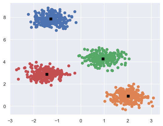
WebアプリのためのExcelデータの生成
Webアプリで用いるExcelのデータをcsvファイルから生成する.
需要予測データ
- 需要データ: demand_with_promo
- プロモーションデータ: promo
から
- 需要予測用のExcelデータ: forecast_small.xlsx
を生成する.
#for forecast
folder = "../data/"
fns = ["demand_with_promo", "promo"]
sheet_name =["demand_with_promo", "promo"]

df ={}
for fn in fns:
    df[fn] = pd.read_csv(folder+fn+".csv", index_col=0)
    df[fn] = df[fn].iloc[:100,:]

with pd.ExcelWriter('forecast_small.xlsx') as writer:
    for i,fn in enumerate(fns):
        df[fn].to_excel(writer, sheet_name=sheet_name[i], index=False)
SCBASデータ
- 需要データ: demand
- 製品データ: prod_for_scbas
から
- SCBAS用のExcelデータ: scbas.xlsx
を生成する.
# for scbas
folder = "../data/"
fns = ["demand", "prod_for_scbas"]
df ={}
for fn in fns:
    df[fn] = pd.read_csv(folder+fn+".csv", index_col=0)
with pd.ExcelWriter('scbas.xlsx') as writer:
    for fn in fns:
        df[fn].to_excel(writer, sheet_name=fn)
MELOS-GFデータ
- 施設データ: melos-gf
- 移動時間データ: time
から
- MELOS-GF用のExcelデータ: melos-gf.xlsx
を生成する.
#for melos-gf
folder = "../data/melos/"
fns = ["melos-gf", "time"]
df ={}
for fn in fns:
    df[fn] = pd.read_csv(folder+fn+".csv",index_col=0)
with pd.ExcelWriter('melos-gf.xlsx') as writer:
    for fn in fns:
        df[fn].to_excel(writer, sheet_name=fn, index=False)
MELOSデータ
- 顧客データ: Cust
- 製品データ: Prod
- 需要データ: demand
- 倉庫データ: DC
- 工場データ: Plnt
- 工場・製品データ: Plnt-Prod
- 移動時間データ: time
から
- MELOS用のExcelデータ: melos.xlsx
を生成する.
#for melos
folder = "../data/"
fns = ["Cust", "Prod", "demand", "DC", "Plnt", "Plnt-Prod", "time"]
df ={}
for fn in fns:
    df[fn] = pd.read_csv(folder+fn+".csv", index_col=0)
with pd.ExcelWriter('melos.xlsx') as writer:
    for fn in fns:
        df[fn].to_excel(writer, sheet_name=fn, index=False)
MESSAデータ
- 在庫地点(段階)データ: ssa01
- 部品展開表データ: ssa_bom01
から
- MESSA用のExcelデータ: messa.xlsx
を生成する.
#for messa
folder = "../data/bom/"
fns = ["ssa01", "ssa_bom01"]
sheet_name =["stage", "bom"]
df ={}
for fn in fns:
    df[fn] = pd.read_csv(folder+fn+".csv", index_col=0)
with pd.ExcelWriter('messa.xlsx') as writer:
    for i,fn in enumerate(fns):
        df[fn].to_excel(writer, sheet_name=sheet_name[i], index=False)
OptSeqデータ
- act: 作業データ
- res: 資源データ
- mode: モードデータ
- act_mode: 作業・モードデータ
- mode_res: モード・資源データ
- temp: 時間制約データ
- non_res : 再生不能資源の右辺定数と制約の向きを表すデータ
- non_lhs : 再生不能資源の項(係数、作業、モードの組)を表すデータ
- state : 状態データ
から
- OptSeq用のExcelデータ: optseq.xlsx
を生成する.
#for optseq
folder = "../data/optseq/"
name ="ex22_"
fns = ["act","mode", "res", "act_mode", "mode_res", "temp", "non_res", "non_lhs", "state" ]
df ={}
for i in fns:
    fn =name+i
    df[fn] = pd.read_csv(folder+fn+".csv", index_col=1)
    df[fn].drop("Unnamed: 0", axis=1, inplace=True)
with pd.ExcelWriter('optseq.xlsx') as writer:
    for i in fns:
        fn =name+i
        df[fn].to_excel(writer, sheet_name=i)
METROデータ
- node: 作業データ
- job: 資源データ
- vehicle: モードデータ
- shipment: 作業・モードデータ
- break: モード・資源データ
- 移動時間データ: time
から
- METRO用のExcelデータ: metro.xlsx
を生成する.
#for metro
folder = "../data/metroIV/"
fns = ["node", "job", "vehicle", "shipment", "break", "time"]
df ={}
for fn in fns:
    if fn =="break":
        df[fn] = pd.read_csv(folder+fn+".csv", index_col=1)
    else:
        df[fn] = pd.read_csv(folder+fn+"02.csv", index_col=1)
    df[fn].drop("Unnamed: 0", axis=1, inplace=True)
with pd.ExcelWriter('metro.xlsx') as writer:
    for fn in fns:
        df[fn].to_excel(writer, sheet_name=fn)
OptShiftデータ
- period : 期間データフ
- break : 休憩データ
- day : 日データ
- job : ジョブデータ
- staff : スタッフデータ
- requirement : 必要人数データ
から
- OptShift用のExcelデータ: optshift.xlsx
を生成する.
#for optshift
folder = "../data/shift/"
fns = ["period", "break", "day", "job", "staff", "requirement"]
df ={}
for fn in fns:
    df[fn] = pd.read_csv(folder+fn+".csv", index_col=1)
    df[fn].drop("Unnamed: 0", axis=1, inplace=True)
with pd.ExcelWriter('optshift.xlsx') as writer:
    for fn in fns:
        df[fn].to_excel(writer, sheet_name=fn)
OptLotデータ
- lotprod: 製品データ
- production : 生産情報データ
- bom : 部品展開表データ
- plnt-demand : 工場における(期別・製品別の)需要を入れたデータ
- resource : 資源データ
から
- OptLot用のExcelデータ: optlot.xlsx
を生成する.
SENDOデータ
- DC: 施設(倉庫)データ
- od: 需要(OD)データ
から
- SENDO用のExcelデータ: sendo.xlsx
を生成する.
#hide ## 郵便番号一覧から離島を削除
顧客データのランダム生成関数 generate_cust
日本の郵便番号データからランダムに地点をサンプリングすることによって、仮想の顧客データを生成する。 社名はFakeパッケージを用いて生成する。 配送計画問題の例題を作成する場合は、あまり遠い地点を選ばないように、都道府県名を引数 prefecture で指定する。 例えば、ロジスティクス・ネットワーク設計モデルやサービスネットワーク設計モデルにおいては、日本全国からランダムに選択し、配送計画モデルにおいては1つの県から選択する。
引数:
- num_locations: 地点数
- random_seed: 乱数の種(同じ問題例が欲しい場合には、同じ種を与える。)
- prefecture: 都道府県名(例えば”千葉県”のような文字列で与える。)省略するか空白の文字列の場合には、日本全国から選択する。
- no_island: 元になる郵便番号データから離島を除いたものを使う場合 True (既定値)
返値:
- ランダムに生成された顧客データ
データの列で必須なものは,名前 (name) と緯度・経度 (lat, lon; latitude, Longitudeの略) があれば良いが、リアリティを出すために,郵便番号と住所情報も付加されているが,最適化で必要な列は以下のものだけである.
顧客データの列:
- name: 名称
- lat: 緯度
- lon: 経度
generate_cust
def generate_cust(
    num_locations:int=10, random_seed:int=1, prefecture:NoneType=None, no_island:bool=True
):
顧客データをランダムに生成する関数
generate_cust の使用例
cust_df = generate_cust(num_locations = 1000, random_seed = 1, prefecture = None, no_island=True)
#cust_df.to_csv(folder+"case/cust100.csv")
cust_df.head()| zip | 都道府県 | 市区町村 | 大字 | lat | lon | name | |
|---|---|---|---|---|---|---|---|
| 0 | 6330253 | 奈良県 | 宇陀市 | 榛原萩原 | 34.538739 | 135.951724 | 合同会社前田建設 第 31 支店 |
| 1 | 4670014 | 愛知県 | 名古屋市瑞穂区 | 白羽根町 | 35.127132 | 136.937726 | 有限会社阿部運輸 第 69 支店 |
| 2 | 9860103 | 宮城県 | 石巻市 | 中島 | 38.533093 | 141.335295 | 株式会社村上印刷 第 51 支店 |
| 3 | 893333 | 北海道 | 中川郡本別町 | 山手町 | 43.128300 | 143.616592 | 佐藤印刷合同会社 第 20 支店 |
| 4 | 3220041 | 栃木県 | 鹿沼市 | 三幸町 | 36.560454 | 139.742275 | 合同会社青木水産 第 85 支店 |
地点間の距離が小さい顧客同士を列挙する関数 enumerate_near_points
同じ緯度・経度をもつ点があると,不具合を起こす場合があるので,事前に確認する関数を準備しておく.
引数: - cust_df: 顧客データフレーム - max_dis: 緯度経度を座標としたときの直線距離の上限;この値以下の地点の対を列挙する.
返値: - 近い点同士の情報を入れたデータフレーム
enumerate_near_points
def enumerate_near_points(
    cust_df, max_dis:float
):
地点間の距離が小さい顧客同士を列挙する関数 enumerate_near_points
df = enumerate_near_points(cust_df, 0.001)
df.head()| point1 | point2 | Euclidean distance | Great circle distance | |
|---|---|---|---|---|
| 0 | 合同会社山崎情報 第 93 支店 | 有限会社佐藤水産 第 57 支店 | 0.0 | 0.0 km |
| 1 | 株式会社藤原鉱業 第 54 支店 | 長谷川鉱業有限会社 第 25 支店 | 0.0 | 0.0 km |
| 2 | 長谷川水産株式会社 第 98 支店 | 有限会社田中銀行 第 40 支店 | 0.0 | 0.0 km |
| 3 | 合同会社林電気 第 86 支店 | 株式会社田中水産 第 40 支店 | 0.0 | 0.0 km |
| 4 | 斎藤食品合同会社 第 66 支店 | 有限会社山下鉱業 第 49 支店 | 0.0 | 0.0 km |
顧客データの読み込み
顧客データをランダムに生成すると、リアリティがないデータになる危険性が高い。 日本全体にまんべんなく散りばめた顧客データが欲しい場合には、あらかじめ準備されたデータを用いる。 ここでは、各県の県庁所在地に顧客がいると仮定したデータを用いる。
ファイル名はCust.csvであり、データの列は、名前 (name) と緯度・経度 (lat, lon; latitude, longitudeの略) である。
import pandas as pd
cust_df = pd.read_csv(folder+"Cust.csv", index_col="id")
cust_df.head()| name | lat | lon | |
|---|---|---|---|
| id | |||
| 1 | 札幌市 | 43.06417 | 141.34694 |
| 2 | 青森市 | 40.82444 | 140.74000 |
| 3 | 盛岡市 | 39.70361 | 141.15250 |
| 4 | 仙台市 | 38.26889 | 140.87194 |
| 5 | 秋田市 | 39.71861 | 140.10250 |
#hide ## ProfileReportの作成
pandas_profilingでデータフレームのレポートを作成する.
https://pandas-profiling.github.io/pandas-profiling/docs/master/rtd/index.html
使用例
profile = ProfileReport(large_dataset, minimal=True)
profile.to_file("output.html")
#hide ## データベースへの保存
Mongodb Atlas server https://cloud.mongodb.com/ を用いる. 会社のメイルでログイン, 512Mまで無料.
Mongoengine (Object Document http://mongoengine.org/ で接続.
pip (pipenv) でインストールできる. dnspythonも同時に入れる必要がある.
以下のようにクラスでドキュメントを定義する.
class User(Document):
    email = EmailField(required=True, unique = True)
    first_name = StringField(max_length=50)
    last_name = StringField(max_length=50)
    password = StringField(min_length = 8, max_length=50)
もしくはpymongoで,データフレームをそのままクライアントに保存する.
これが一番簡単だが,プロジェクト形式で,複数のデータフレームをまとめておくことができない.
#hide ### データベースのコレクション(ドキュメントのリスト)からの読み込み
#collection_names = db.list_collection_names()#hide ## データベースからの読み込み
#hide ## 中国の配送計画問題用の顧客データとトラックデータの生成
顧客の可視化関数 plot_cust
可視化モジュールPlotlyを使うと、顧客を地図上に表示できる。
引数: - cust_df: 顧客データフレーム - weight: 顧客の重み(需要量や売上)を表す配列;この量によって点の大きさを変えて描画する. (既定値はNoneで,その場合には同じ大きさで描画する.)
返値: - fig: Plotlyの図オブジェクト
plot_cust
def plot_cust(
    cust_df, weight:NoneType=None
):
顧客データフレームを入れると、PlotlyのFigureオブジェクトに地図を入れて返す関数
plot_cust 関数の使用例
上のplot_cust関数の適用例を示す。
total_demand_df = pd.read_csv(folder+"total_demand.csv")
demand_df = pd.pivot_table(total_demand_df, index="cust",values="demand")
cust_df = pd.read_csv(folder+"Cust.csv")
fig = plot_cust(cust_df, demand_df.demand)
plotly.offline.plot(fig);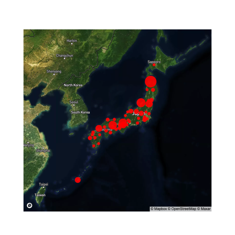
製品データの生成関数 generate_prod, generate_many_prod
製品名は仮想のデータとし、大文字のアルファベットとする.
製品名をA,B,C...とする場合には,26以下の整数を製品数num_prodに指定する(generate_prod).より大きい問題例の場合には,製品名を”prod1”のように数字をつけて表す(generate_many_prod).
基本となる製品は、以下のデータをもつ。
- weight: 製品の重量を表す。これは引数 weight_bound (下限と上限のタプル) 間の一様乱数によって生成された整数とする。 (単位重量)
- volume: 製品の容積を表す。これは引数 volume_bound (下限と上限のタプル) 間の一様乱数によって生成された整数とする。(単位容積)
- cust_value : 顧客上での製品の価値を表す。これは引数 cust_value_bound (下限と上限のタプル) 間の一様乱数によって生成された整数とする。(円)
- dc_value : 倉庫上での製品の価値を表す。これは引数 dc_value_bound (下限と上限のタプル) 間の一様乱数によって生成された整数とする。(円)
- plnt_value : 工場における製品の価値を表す。これは引数 plnt_value_bound (下限と上限のタプル) 間の一様乱数によって生成された整数とする。(円)
- fixed_cost: 製品の生産固定費用を表す。これは引数fc_bound (下限と上限のタプル) 間の一様乱数によって生成された整数とする。(円/回)
引数: - num_prod: 製品数(generate_prodの場合は26以下の整数) - weight_bound: 製品の重量を生成するための下限と上限のタプル - volume_bound: 製品の容積を生成するための下限と上限のタプル - cust_value_bound: 顧客上での製品の価値を生成するための下限と上限のタプル - dc_value_bound: 倉庫上での製品の価値を生成するための下限と上限のタプル - plnt_value_bound: 工場における製品の価値を生成するための下限と上限のタプル - fc_bound: 製品の生産固定費用生成のための下限と上限のタプル - random_seed: 乱数の種
返値: - 製品データフレーム
列名: - name: 製品の名称 - weight: 製品の重量 (単位はkg) - volume: 製品の容量 (単位は \(m^3\)) - cust_value: 顧客上での製品の価値 - dc_value: 倉庫上での製品の価値 - plnt_value: 工場における製品の価値 - fixed_cost: 製品を生産する際の段取り(固定)費用
generate_prod
def generate_prod(
    num_prod:int=10, weight_bound:tuple=(0, 0), volume_bound:tuple=(0, 0), cust_value_bound:tuple=(1, 1),
    dc_value_bound:tuple=(1, 1), plnt_value_bound:tuple=(1, 1), fc_bound:tuple=(1, 1), random_seed:int=1
):
仮想の製品のデータフレームを生成する関数
generate_many_prod
def generate_many_prod(
    num_prod:int=100, weight_bound:tuple=(0, 0), volume_bound:tuple=(0, 0), cust_value_bound:tuple=(1, 1),
    dc_value_bound:tuple=(1, 1), plnt_value_bound:tuple=(1, 1), fc_bound:tuple=(1, 1), random_seed:int=1
):
仮想の製品のデータフレーム(26より大きい)を生成する関数
generate_prod関数の使用例
10個の製品をそれらの重量を1以上5以下の整数に、顧客上での価値は5以上10以下の整数に、容積と他の価値は既定値、生産固定費用を10以上20以下の整数になるように設定する。
prod_df = generate_prod(10, weight_bound=(1, 5), cust_value_bound =(5,10), fc_bound=(10,20))
#prod_df.to_csv(folder+"Prod.csv")
prod_df.head()| name | weight | volume | cust_value | dc_value | plnt_value | fixed_cost | |
|---|---|---|---|---|---|---|---|
| 0 | A | 2 | 0 | 7 | 1 | 1 | 14 |
| 1 | B | 5 | 0 | 5 | 1 | 1 | 14 |
| 2 | C | 1 | 0 | 5 | 1 | 1 | 19 |
| 3 | D | 3 | 0 | 5 | 1 | 1 | 17 |
| 4 | E | 1 | 0 | 10 | 1 | 1 | 18 |
#prod_df = generate_many_prod(num_prod=100, weight_bound=(0, 0), volume_bound=(0, 10), cust_value_bound=(1, 10))
#prod_df.head()| name | weight | volume | cust_value | dc_value | plnt_value | fixed_cost | |
|---|---|---|---|---|---|---|---|
| 0 | prod0 | 0 | 10 | 3 | 1 | 1 | 1 |
| 1 | prod1 | 0 | 2 | 10 | 1 | 1 | 1 |
| 2 | prod2 | 0 | 8 | 9 | 1 | 1 | 1 |
| 3 | prod3 | 0 | 9 | 1 | 1 | 1 | 1 |
| 4 | prod4 | 0 | 2 | 7 | 1 | 1 | 1 |
需要データの生成関数 generate_demand
顧客データと製品データを与えると、仮想の需要データを生成する関数を準備しておく。 需要は、以下のパラメータを用いて生成される。基本的な分布はパレート分布とし、週次ならびに月次の波動と誤差項を加える。
引数: - cust_df: 顧客データフレーム - prod_df: 製品データフレーム - cust_shape: 顧客のパレート分布の形状を定める定数 (正の値であり,小さいほど分布が偏る.) - prod_shape: 製品のパレート分布の形状を定める定数 (正の値であり,小さいほど分布が偏る.) - weekly_ratio: 週次の波動を表すリスト(0が日曜日);長さは7 - yearly_ratio: 年次の波動を表すリスト(0が1月);長さは12 - start: 開始日 - periods: 計画期間数 - epsilon: 誤差項の標準偏差 - random_seed: 乱数の種
返値: - demand_df: 需要データフレーム
列名: - date: 日付 - cust: 顧客名 - prod: 製品名 - demand: 需要量
generate_demand
def generate_demand(
    cust_df, prod_df, cust_shape:float=1.7, prod_shape:float=1.7, weekly_ratio:list=[1, 1, 1, 1, 1, 1, 1],
    yearly_ratio:list=[1, 1, 1, 1, 1, 1, 1, 1, 1, 1, 1, 1], start:str='2019/01/01', periods:int=365,
    epsilon:float=0.0, random_seed:int=1
):
ランダムな需要を生成する関数
generate_demand関数の使用例
weekly_ratio = [1.0, 1.0, 1.2, 1.3, 0.9, 1.5, 0.2]  # 0 means Sunday
yearly_ratio = [1.0 + np.sin(i) for i in range(13)]  # 0 means January
demand_df = generate_demand(cust_df, prod_df, cust_shape=1.7, prod_shape=1.6, weekly_ratio=weekly_ratio, yearly_ratio=yearly_ratio,
                            start="2019/01/01", periods=365, epsilon=1.)
#demand_df.to_csv(folder + "demand_all.csv")
demand_df.head()generate_demand_normal
def generate_demand_normal(
    cust_df, prod_df, cust_loc, cust_scale, prod_loc, prod_scale, weekly_ratio:list=[1, 1, 1, 1, 1, 1, 1],
    yearly_ratio:list=[1, 1, 1, 1, 1, 1, 1, 1, 1, 1, 1, 1], start:str='2019/01/01', periods:int=365,
    epsilon:float=0.0, random_seed:int=1
):
ランダムな正規分布の需要を生成する関数
generate_demand_normal関数の使用例
weekly_ratio = [1.1, 1.2, 1.0, 0.9, 0.8, 0.95, 1.0]  # 0 means Sunday
yearly_ratio = [1.0 + 0.1*np.sin(i) for i in range(13)]  # 0 means January
demand_df = generate_demand_normal(cust_df, prod_df, cust_loc=100., cust_scale=10, prod_loc=10., prod_scale=4., weekly_ratio=weekly_ratio, yearly_ratio=yearly_ratio,
                            start="2019/01/01", periods=365, epsilon=100.)
demand_df.to_csv(folder + "demand_normal.csv")
demand_df.head()| date | cust | prod | demand | |
|---|---|---|---|---|
| 0 | 2019-01-01 | 札幌市 | A | 2695 |
| 1 | 2019-01-01 | 札幌市 | B | 1606 |
| 2 | 2019-01-01 | 札幌市 | C | 1745 |
| 3 | 2019-01-01 | 札幌市 | D | 1485 |
| 4 | 2019-01-01 | 札幌市 | E | 1089 |
プロモーション情報の生成とプロモーションを加味した需要の生成関数 generate_demand_with_promo
引数: - cust_df: 顧客データフレーム - prod_df: 製品データフレーム - promo_df: プロモーション情報を入れたデータフレーム(promo_dfは、需要と同じ日付を入れた列dateと、プロモーション名を列名とし、その効果を列データとした列を持つものとする。) - cust_shape: 顧客のパレート分布の形状を定める定数 - prod_shape: 製品のパレート分布の形状を定める定数 - weekly_ratio: 週次の波動を表すリスト(0が日曜日);長さは7 - yearly_ratio: 年次の波動を表すリスト(0が1月);長さは12 - start: 開始日 - periods: 計画期間数 - epsilon: 誤差項の標準偏差
返値: - demand_df: プロモーション情報を加味した需要データフレーム
generate_demand_with_promo
def generate_demand_with_promo(
    cust_df, prod_df, promo_df, cust_shape:float=1.7, prod_shape:float=1.7, weekly_ratio:list=[1, 1, 1, 1, 1, 1, 1],
    yearly_ratio:list=[1, 1, 1, 1, 1, 1, 1, 1, 1, 1, 1, 1], start:str='2019/01/01', periods:int=365,
    epsilon:float=0.0
):
プロモーション情報を加味したランダムな需要を生成する関数
generate_demand_with_promo関数の使用例
プロモーション情報を加えた需要データを生成しておく。プロモーション情報は、promo_dfデータフレームに保管してあるものとする。
promo_dfは、需要と同じ日付を入れた列dateと、プロモーション名を列名とし、その効果を列データとした列を持つものとする。
start="2019/01/01"
periods =365*3
date_col = []
num_promo =2
promo_cols = [ [] for promo_ in range(num_promo)]
for t in pd.date_range(start, periods=periods):
    date_col.append(t)
    if t.weekday() == 2:  # Tsuesday promotion
        promo_cols[0].append(1)
    else:
        promo_cols[0].append(0)
    if t.day%10 ==0: # 10th, 20th 30th day promotion
        promo_cols[1].append(1)
    else:
        promo_cols[1].append(0)

promo_df = pd.DataFrame(data={"date": date_col, "promo_0": promo_cols[0], "promo_1": promo_cols[1]})
#promo_df.head(20)
#promo_df.to_csv(folder + "promo.csv")
promo_df.head()| date | promo_0 | promo_1 | |
|---|---|---|---|
| 0 | 2019-01-01 | 0 | 0 |
| 1 | 2019-01-02 | 1 | 0 |
| 2 | 2019-01-03 | 0 | 0 |
| 3 | 2019-01-04 | 0 | 0 |
| 4 | 2019-01-05 | 0 | 0 |
weekly_ratio = [0.1, 1.0, 1.2, 1.3, 0.9, 1.5, 0.2]  # 0 means Sunday
yearly_ratio = [1.0 + np.sin(i) for i in range(13)]  # 0 means January
demand_with_promo_df = generate_demand_with_promo(cust_df[:], prod_df[:], promo_df, cust_shape=1.7, prod_shape=1.6, weekly_ratio=weekly_ratio, yearly_ratio=yearly_ratio,
                            start="2019/01/01", periods=365*2, epsilon=1.)
#demand_with_promo_df.to_csv(folder + "demand_with_promo_all.csv")demand_with_promo_df.tail()| date | cust | prod | promo_0 | promo_1 | demand | |
|---|---|---|---|---|---|---|
| 21895 | 2020-12-30 | 宇都宮市 | B | 1 | 1 | 0 |
| 21896 | 2020-12-30 | 宇都宮市 | C | 1 | 1 | 6 |
| 21897 | 2020-12-30 | 前橋市 | A | 1 | 1 | 3 |
| 21898 | 2020-12-30 | 前橋市 | B | 1 | 1 | 0 |
| 21899 | 2020-12-30 | 前橋市 | C | 1 | 1 | 4 |
予約需要の生成関数 generate_reservation_demand
収益管理で用いるランダムな予約需要データフレームを生成する。
引数: - class_df: 予約のクラスを表すデータフレーム; class_name列と基本需要(Possion分布に与える平均需要)を表す列 basic_demandをもつ。 - weekly_ratio: 週次の波動を表すリスト(0が日曜日);長さは7 - start: 開始日 - periods: 計画期間数 - max_lt: 予約可能な日が何日前かを表すパラメータ
返値: - reserve_demand_df: 予約需要データフレーム
generate_reservation_demand
def generate_reservation_demand(
    class_df, weekly_ratio:list=[1, 1, 1, 1, 1, 1, 1], start:str='2019/01/01', periods:int=7, max_lt:int=1
):
ランダムな予約需要を生成する関数
generate_reservation_demand関数の使用例
if TEST:
    class_df = pd.DataFrame({"class_name":["C","B","A"], "basic_demand": [20, 10, 5]})
    weekly_ratio = [0.0, 1.0, 1.2, 1.3, 0.9, 1.5, 0.2]  # 0 means Sunday
    start="2019/01/01"
    periods = 60
    max_lt = 30 # reservation in starts max_lt before check-in day
    reserve_demand_df = generate_reservation_demand(class_df, weekly_ratio=[1]*7, start="2019/01/01", periods=7, max_lt = 1)
    reserve_demand_df.to_csv(folder+"reserve_demand.csv")
reserve_demand_df.head()| reserve | checkin | class_name | demand | |
|---|---|---|---|---|
| 0 | 2019-01-01 | 2019-01-02 | C | 14 |
| 1 | 2019-01-01 | 2019-01-02 | B | 6 |
| 2 | 2019-01-01 | 2019-01-02 | A | 5 |
| 3 | 2019-01-02 | 2019-01-02 | C | 19 |
| 4 | 2019-01-02 | 2019-01-02 | B | 8 |
OD需要量の生成
サービスネットワーク設計問題に対しては、地点間の需要量を定義する必要がある。荷物の始点を発生地点(origin)、終点を集中地点(destination)と呼ぶ。 地点間の需要量は、ODフロー量と呼ばれる。
ここでは、重力法 (gravity method) を用いて需要量を算出する。 県別の人口を入れた顧客データを読み込み、以下の式によって地点 \(i\) から地点 \(j\) へのODフロー量を計算する。
記号: - \(P_i\) : 地点 \(i\) の人口 - \(d_{ij}\) : 地点 \(i,j\) 間の距離(ここでは大圏距離とする。) - \(D_{ij}\) : 地点 \(i,j\) 間のODフロー量 - \(\alpha\) : 発生地点の人口がODフロー量に与える影響度 - \(\beta\) : 集中地点の人口がODフロー量に与える影響度
重力法: \[ D_{ij}= P_i^{\alpha} P_j^{\beta}/d_{ij} \]
都道府県の人口を入れたデータCust_with_population.csvを読み込む。
# #人口データの付加
# cust_df = pd.read_csv(folder+"Cust.csv", index_col=0)
# pop_df = pd.read_csv("population.csv")
# cust_df.reset_index(inplace=True)
# cust_df["population"] = pop_df["pop"].str.replace(",","").astype(float)
# cust_df.to_csv(folder + "Cust_with_population.csv")
cust_df = pd.read_csv(folder+"Cust_with_population.csv", index_col=0)
cust_df.head()| id | name | lat | lon | population | |
|---|---|---|---|---|---|
| 0 | 1 | 札幌市 | 43.06417 | 141.34694 | 5320.0 |
| 1 | 2 | 青森市 | 40.82444 | 140.74000 | 1278.0 |
| 2 | 3 | 盛岡市 | 39.70361 | 141.15250 | 1255.0 |
| 3 | 4 | 仙台市 | 38.26889 | 140.87194 | 2323.0 |
| 4 | 5 | 秋田市 | 39.71861 | 140.10250 | 996.0 |
n = len(cust_df)
D = np.zeros( (n,n) )
Distance = np.zeros( (n,n) )
alpha, beta = 1.,0.5
for i, row1 in enumerate(cust_df.itertuples()):
    for j, row2 in enumerate(cust_df.itertuples()):
        if i==j:
            D[i,j] = 0.
        else:
            D[i,j] = (row1.population**alpha) * (row2.population**beta) /great_circle( (row1.lat, row1.lon), (row2.lat,row2.lon)).km
            Distance[i,j] = great_circle( (row1.lat, row1.lon), (row2.lat,row2.lon)).km
od_df = pd.DataFrame(D, index=cust_df.name, columns=cust_df.name)
od_df.head()| name | 札幌市 | 青森市 | 盛岡市 | 仙台市 | 秋田市 | 山形市 | 福島市 | 水戸市 | 宇都宮市 | 前橋市 | ... | 松山市 | 高知市 | 福岡市 | 佐賀市 | 長崎市 | 熊本市 | 大分市 | 宮崎市 | 鹿児島市 | 那覇市 |
|---|---|---|---|---|---|---|---|---|---|---|---|---|---|---|---|---|---|---|---|---|---|
| name | |||||||||||||||||||||
| 札幌市 | 0.000000 | 748.604013 | 503.880787 | 479.530853 | 434.728978 | 325.400616 | 387.515654 | 380.707553 | 320.950984 | 306.975814 | ... | 155.037392 | 113.142207 | 268.320507 | 104.968908 | 128.494480 | 151.969403 | 130.564385 | 115.832932 | 134.674821 | 89.979170 |
| 青森市 | 366.911870 | 0.000000 | 349.739599 | 216.591680 | 300.250555 | 146.736232 | 161.797705 | 137.690614 | 117.949336 | 110.061161 | ... | 45.045703 | 33.190310 | 75.179922 | 29.333277 | 35.666270 | 42.628874 | 37.127441 | 32.597444 | 37.480032 | 24.019524 |
| 盛岡市 | 244.733739 | 346.578201 | 0.000000 | 374.849054 | 440.904081 | 236.165870 | 241.756337 | 178.105294 | 151.641357 | 135.078213 | ... | 46.792775 | 34.814853 | 76.531004 | 29.884567 | 36.305497 | 43.649604 | 38.222610 | 33.627525 | 38.454102 | 24.419156 |
| 仙台市 | 316.873079 | 292.012168 | 509.987066 | 0.000000 | 420.427689 | 1732.062426 | 1488.646715 | 574.094165 | 492.841131 | 390.859150 | ... | 97.623923 | 73.645927 | 154.638886 | 60.388289 | 73.150841 | 88.750941 | 78.475998 | 68.944247 | 78.125318 | 48.416035 |
| 秋田市 | 188.101580 | 265.062360 | 392.782315 | 275.293764 | 0.000000 | 199.309319 | 195.354280 | 142.173921 | 125.495887 | 115.713660 | ... | 39.834352 | 29.538809 | 64.824922 | 25.242764 | 30.545651 | 36.765353 | 32.327894 | 28.150575 | 32.123788 | 19.989013 |
5 rows × 47 columns
#heatmap
#fig = px.imshow(D)
#fig.show()
od_df.to_csv(folder + "od.csv")
#hide ## 実際問題のデータの読み込み
実際問題を解きたい場合には、上と同じ形式のデータを作成して読みこむ。
Plotly Expressによる需要の変化の図示
fig = px.line(demand_df, x="date",  y="demand", color ="prod")
#fig = px.line(demand_with_promo_df, x="date",  y="demand", color ="prod")
#plotly.offline.plot(fig)
Image("../figure/demand_series.png")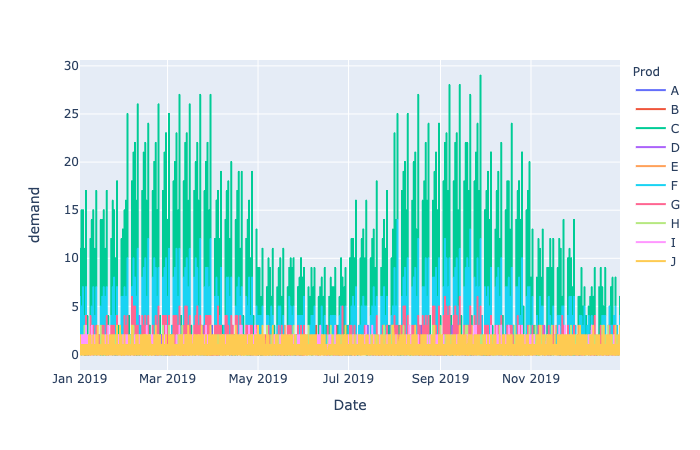
Plotly Expressによる需要のヒストグラムの図示
fig = px.histogram(demand_df, x="demand")
#fig = px.histogram(demand_with_promo_df, x="demand")
#plotly.offline.plot(fig)
Image("../figure/demand_hist.png")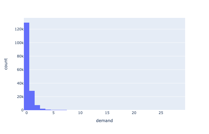
需要の属性を生成する関数 demand_attribute_compute
需要量に応じて、以下のような諸量を計算し、需要データフレームに属性(列)として追加する関数
- 製品の売り上げ: 需要と製品の顧客上での価値(\(=\)価格)の積
- 重量合計:需要量と製品重量の積
- 容積合計:需要量と製品容積の積
引数:
- demand_df : 需要データフレーム
- prod_df : 製品データフレーム
- attribute_col_name : 需要にかけ合わせる製品データの列名;例えば、売り上げを計算したい場合には “cust_value” とする。
- new_col_name : 計算結果を格納するための列名;例えば、売り上げを保管したい場合には “sales” とする。
返値:
- 新しい列を追加した需要データフレーム
demand_attribute_compute
def demand_attribute_compute(
    demand_df, prod_df, attribute_col_name, new_col_name
):
需要データに新たな属性を追加する関数
demand_attribute_compute関数の使用例
demand_df = demand_attribute_compute(demand_df, prod_df, "cust_value", "sales")
#demand_df.to_csv(folder + "demand.csv")
demand_df.head()| date | cust | prod | demand | sales | |
|---|---|---|---|---|---|
| 0 | 2019-01-01 | 札幌市 | A | 1 | 7 |
| 1 | 2019-01-01 | 札幌市 | B | 1 | 5 |
| 2 | 2019-01-01 | 札幌市 | C | 0 | 0 |
| 3 | 2019-01-01 | 札幌市 | D | 0 | 0 |
| 4 | 2019-01-01 | 札幌市 | E | 0 | 0 |
倉庫データの生成関数 generate_dc
倉庫の開設可能地点は、全ての顧客上と仮定する。 製品ごとの需要に製品の重量 weight を乗じたものの合計を計算し、それを倉庫の予定開設個数で割ることによって、倉庫の容量を設定する。 倉庫の容量の下限と上限を決める率 lb_ratio, ub_ratio を乗じて、下限と上限を決める。
引数: - cust_df: 顧客データフレーム - demand_df: 需要データフレーム - prod_df: 製品データフレーム - num_dc =5: 目標とする倉庫数(これにあわせて容量を決める. - lb_ratio=0.8: 容量の下限を決めるパラメータ - ub_ratio =1.2: 容量の上限を決めるパラメータ - vc_bound =(0.,0.5): 変動費用の下限と上限を表すパラメータ - fc_bound =(10000,10000): 固定費用の下限と上限を表すパラメータ - random_seed: 乱数の種
返値のデータフレームの列名と意味は以下の通り.
- name: 倉庫名称
- lb: 容量下限
- ub: 容量上限
- fc: 固定費用
- vc: 変動費用
- lat: 緯度
- lon: 経度
generate_dc
def generate_dc(
    cust_df, demand_df, prod_df, num_dc:int=5, lb_ratio:float=0.8, ub_ratio:float=1.2, vc_bounds:tuple=(0.0, 0.5),
    fc_bounds:tuple=(10000, 11000), random_seed:int=1
):
倉庫データの生成: 顧客データ、需要データ、製品データ、予定開設数、倉庫の容量を決めるための下限率、上限率を与えると、倉庫データを返す。
generate_dc関数の使用例
demand_df = pd.read_csv(folder+"demand.csv")
dc_df = generate_dc(cust_df, demand_df, prod_df, num_dc=5, lb_ratio=0.0, ub_ratio=10.3)
dc_df.to_csv(folder + "DC.csv")
dc_df.head()| name | lb | ub | fc | vc | lat | lon | |
|---|---|---|---|---|---|---|---|
| 0 | 札幌市 | 0.0 | 501136.2 | 10037 | 0.432510 | 43.06417 | 141.34694 |
| 1 | 青森市 | 0.0 | 501136.2 | 10235 | 0.414573 | 40.82444 | 140.74000 |
| 2 | 盛岡市 | 0.0 | 501136.2 | 10908 | 0.414802 | 39.70361 | 141.15250 |
| 3 | 仙台市 | 0.0 | 501136.2 | 10072 | 0.136525 | 38.26889 | 140.87194 |
| 4 | 秋田市 | 0.0 | 501136.2 | 10767 | 0.029622 | 39.71861 | 140.10250 |
工場データと生産情報データの生成関数 generate_plnt
工場は3つで、小田原、大阪、千葉にあると仮定する。 大阪工場では約半分の製品を、千葉では大阪工場で製造していない約半分の製品を生産でき、小田原工場では全ての製品を生産できるものとする。 生産容量は、総需要量と設定しておく。
引数:
- prod_df : 製品データフレーム
- demand_df : 需要データフレーム
- lead_time_bound: 工場での生産リード時間を決めるためのパラメータ; タプルで与えた下限と上限の間の一様整数乱数とする。
返値:
- plnt_df: 工場データフレーム
- plnt_prod_df: 工場・製品データフレーム
generate_plnt
def generate_plnt(
    prod_df, demand_df, lead_time_bound:tuple=(1, 2), random_seed:int=1
):
工場データの生成
generate_plnt関数の使用例
prod_df = pd.read_csv(folder+"Prod.csv")
demand_df = pd.read_csv(folder+"demand.csv")
plnt_df, plnt_prod_df = generate_plnt(prod_df, demand_df, lead_time_bound=(25,30))
plnt_df.to_csv(folder + "Plnt.csv")
plnt_df.head()| name | lat | lon | |
|---|---|---|---|
| 0 | Odawara | 35.284982 | 139.196133 |
| 1 | Osaka | 34.563101 | 135.415129 |
| 2 | Chiba | 35.543452 | 140.113908 |
plnt_prod_df.to_csv(folder + "Plnt-Prod.csv")
plnt_prod_df.head()| plnt | prod | ub | lead_time | |
|---|---|---|---|---|
| 0 | Osaka | D | 813 | 28 |
| 1 | Osaka | A | 18026 | 29 |
| 2 | Osaka | E | 77704 | 25 |
| 3 | Osaka | J | 52907 | 26 |
| 4 | Osaka | G | 15774 | 28 |