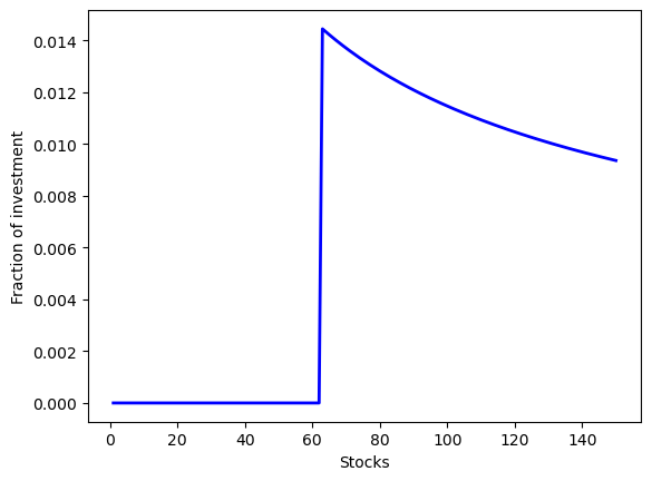
ロバスト最適化

様々なロバスト最適化問題の定式化

ロバストなポートフォリオ

RSOME(Robust Stochastic Optimization Made Easy) パッケージを用いてモデル化する．

モデル

\[ \begin{align} \max~&\min\limits_{\pmb{z}\in\mathcal{Z}} \sum\limits_{i=1}^n\left(p_i + \delta_iz_i \right)x_i \\ \text{s.t.}~&\sum\limits_{i=1}^nx_i = 1 \\ &x_i \geq 0, ~\forall i = 1, 2, ..., n, \end{align} \]

不確実性集合

• 無限大ノルムが \(1\) 以下: 絶対値が \(1\) 以下； 最大値が \(1\)， 最小値が\(-1\)

• \(1\) ノルムが \(\Gamma\) 以下： 各成分の絶対値の和が \(\Gamma\) 以下

\[ \begin{align} \mathcal{Z} = \left\{\pmb{z}: \|\pmb{z}\|_{\infty} \leq 1, \|\pmb{z}\|_1 \leq \Gamma\right\}, \end{align} \]

パラメータ

\[ \begin{align} & \Gamma = 5 &\\ & p_i = 1.15 + i\frac{0.05}{150}, &\forall i = 1, 2, ..., n \\ & \delta_i = \frac{0.05}{450}\sqrt{2 \cdot i \cdot n \cdot (n+1)}, &\forall i = 1, 2, ..., n. \end{align} \]

from rsome import ro
from rsome import grb_solver as grb
import rsome as rso
import numpy as np


n = 150                                 # number of stocks
i = np.arange(1, n+1)                   # indices of stocks
p = 1.15 + i*0.05/150                   # mean returns
delta = 0.05/450 * (2*i*n*(n+1))**0.5   # deviations of returns
Gamma = 5                               # budget of uncertainty

model = ro.Model()              
x = model.dvar(n)                       # fractions of investment
z = model.rvar(n)                       # random variables

model.maxmin((p + delta*z) @ x,         # the max-min objective
             rso.norm(z, np.infty) <=1, # uncertainty set constraints
             rso.norm(z, 1) <= Gamma)   # uncertainty set constraints
model.st(sum(x) == 1)                   # summation of x is one
model.st(x >= 0)                        # x is non-negative

model.solve(grb)                        # solve the model by Gurobi

Restricted license - for non-production use only - expires 2025-11-24
Being solved by Gurobi...
Solution status: 2
Running time: 0.0032s

import matplotlib.pyplot as plt

obj_val = model.get()                   # the optimal objective value
x_sol = x.get()                         # the optimal investment decision

plt.plot(range(1, n+1), x_sol, linewidth=2, color='b')
plt.xlabel('Stocks')
plt.ylabel('Fraction of investment')
plt.show()
print('Objective value: {0:0.4f}'.format(obj_val))

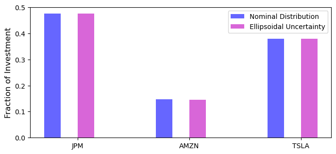
Objective value: 1.1709

CVaR最小化のポートフォリオ

\[ \begin{align} \min~&\max\limits_{\pmb{\pi}\in \Pi} \alpha + \frac{1}{1-\beta}\pmb{\pi}^{\top}\pmb{u} &\\ \text{s.t.}~& u_k \geq -\pmb{y}_k^{\top}\pmb{x} - \alpha, &\forall k = 1, 2, ..., s \\ &u_k \geq 0, &\forall k=1, 2, ..., s \\ &\sum\limits_{k=1}^s\pi_k\pmb{y}_k^{\top}\pmb{x} \geq \mu, &\forall \pmb{\pi} \in \Pi \\ &\underline{\pmb{x}} \leq \pmb{x} \leq \overline{\pmb{x}} \\ &\pmb{1}^{\top}\pmb{x} = w_0 \end{align} \]

不確実性集合がない場合： すべてのサンプルが同じ確率で発生するので， \(\pi\) は \(1/s\) （\(s\) はサンプルの数）と設定する．

不確実性集合が楕円の場合： \[ \Pi = \left\{\pmb{\pi}: \pmb{\pi} = \pmb{\pi}^0 + \rho\pmb{\eta}, \pmb{1}^{\top}\pmb{\eta}=0, \pmb{\pi}^0 + \rho\pmb{\eta} \geq \pmb{0}, \|\pmb{\eta}\| \leq 1 \right\}, \]

import pandas as pd
import yfinance as yf

stocks = ['JPM', 'AMZN', 'TSLA']
start = '2021-1-2'              # starting date of historical data
end='2021-1-31'                # end date of historical data

data = pd.DataFrame([])
for stock in stocks:
    each = yf.Ticker(stock).history(start=start, end=end)
    close = each['Close'].values
    returns = (close[1:] - close[:-1]) / close[:-1]
    data[stock] = returns

data.head()

	JPM	AMZN	TSLA
0	0.005441	0.010004	0.007317
1	0.046956	-0.024897	0.028390
2	0.032839	0.007577	0.079447
3	0.001104	0.006496	0.078403
4	0.014924	-0.021519	-0.078214

import numpy as np

y = data.values     # stock data as an array
s, n = y.shape      # s: sample size; n: number of stocks

x_lb = np.zeros(n)  # lower bounds of investment decisions
x_ub = np.ones(n)   # upper bounds of investment decisions

beta =0.95          # confidence interval
w0 = 1              # investment budget
mu = 0.001          # target minimum expected return rate

from rsome import ro

model = ro.Model()

pi = np.ones(s) / s

x = model.dvar(n)
u = model.dvar(s)
alpha = model.dvar()

model.min(alpha + 1/(1-beta) * (pi@u))
model.st(u >= -y@x - alpha)
model.st(u >= 0)
model.st(pi@y@x >= mu)
model.st(x >= x_lb, x <= x_ub, x.sum() == w0)

model.solve(grb)

x_nom = x.get()
model.get()

Being solved by Gurobi...
Solution status: 2
Running time: 0.0004s

0.025662997827474266

from rsome import ro
import rsome as rso

model = ro.Model()

rho = 0.001

eta = model.rvar(s)
uset = (eta.sum() == 0, 1/s + rho*eta >= 0,
        rso.norm(eta) <= 1)
pi = 1/s + rho*eta

x = model.dvar(n)
u = model.dvar(s)
alpha = model.dvar()

model.minmax(alpha + 1/(1-beta) * (pi@u), uset)
model.st(u >= -y@x - alpha)
model.st(u >= 0)
model.st(pi@y@x >= mu)
model.st(x >= x_lb, x <= x_ub, x.sum() == w0)

model.solve(grb)

x_ellip = x.get()
model.get()

Being solved by Gurobi...
Solution status: 2
Running time: 0.0026s

0.02566380123574748

import matplotlib.pyplot as plt

xdata = np.arange(n)
width = 0.15

plt.figure(figsize=(8, 3.5))
plt.bar(xdata - 1.5*width, x_nom, 
        width=width, color='b', alpha=0.6, label='Nominal Distribution')

plt.bar(xdata + 0.5*width, x_ellip, 
        width=width, color='m', alpha=0.6, label='Ellipsoidal Uncertainty')


plt.legend()
plt.ylabel('Fraction of Investment', fontsize=12)
plt.xticks(xdata, data.columns)
plt.show()

適応型ロバスト在庫配置

\[ \mathcal{U}=\left\{\pmb{d}: \pmb{0}\leq \pmb{d} \leq d_{\text{max}}\pmb{e}, \pmb{e}^{\top}\pmb{d} \leq \Gamma\right\}. \]

\[ \begin{align} \min~&\max\limits_{\pmb{d}\in\mathcal{U}} \sum\limits_{i=1}^Nc_ix_i + \sum\limits_{i=1}^N\sum\limits_{j=1}^Nt_{ij}y_{ij} && &\\ \text{s.t.}~&d_i \leq \sum\limits_{j=1}^Ny_{ji} - \sum\limits_{j=1}^Ny_{ij} + x_i, &&i=1, 2, ..., N, & \forall \pmb{d} \in \mathcal{U} \\ &0\leq x_i\leq K_i, &&i = 1, 2, ..., N & \end{align} \]

\[ y_{ij}(\pmb{d}) = y_{ij}^0 + \sum\limits_{k=1}^Ny_{ijk}^dd_k \]

from rsome import ro
import rsome.grb_solver as grb
import numpy as np
import numpy.random as rd
import matplotlib.pyplot as plt

# Parameters of the lot-sizing problem
N = 8
c = 20
dmax = 5
Gamma = N*np.sqrt(N)
xy = 10*rd.rand(2, N)
t = ((xy[[0]] - xy[[0]].T) ** 2
     + (xy[[1]] - xy[[1]].T) ** 2) ** 0.5

model = ro.Model()          # define a model
x = model.dvar(N)           # define location decisions
y = model.ldr((N, N))       # define decision rule as the shifted quantities
d = model.rvar(N)           # define random variables as the demand

y.adapt(d)                  # the decision rule y affinely depends on d

uset = (d >= 0,
        d <= dmax,
        sum(d) <= Gamma)    # define the uncertainty set

# define model objective and constraints
model.minmax((c*x).sum() + (t*y).sum(), uset)
model.st(d <= y.sum(axis=0) - y.sum(axis=1) + x)
model.st(y >= 0)
model.st(x >= 0)
model.st(x <= 20)

model.solve(grb)

Being solved by Gurobi...
Solution status: 2
Running time: 0.0164s

x_star = x.get()
y_star = y.get()
model.get()
#x_star, y_star

516.8804592697848

plt.figure(figsize=(5, 5))
plt.scatter(xy[0], xy[1], c='w', edgecolors='k')
plt.scatter(xy[0], xy[1], s=40*x.get(), c='k', alpha=0.6)
plt.axis('equal')
plt.xlim([-1, 11])
plt.ylim([-1, 11])
plt.grid()
plt.show()

適応型分布ロバストによる新聞売り子モデル

\[ \begin{align} \min~& -\pmb{p}^{\top}\pmb{x} + \sup\limits_{\mathbb{P}\in\mathcal{F}(\theta)}\mathbb{E}_{\mathbb{P}}\left[\pmb{p}^{\top}\pmb{y}(\tilde{s}, \tilde{\pmb{z}}, \tilde{u})\right] && \\ \text{s.t.}~&\pmb{y}(s, \pmb{z}, u) \geq \pmb{x} - \pmb{z} && \forall (\pmb{z}, \pmb{u}) \in \mathcal{Z}_s, ~\forall s \in [S] \\ & \pmb{y}(s, \pmb{z}, u) \geq \pmb{0} && \forall (\pmb{z}, \pmb{u}) \in \mathcal{Z}_s, ~\forall s \in [S]\\ & y_i \in \overline{\mathcal{A}}(\{\{1\}, \{2\}, \dots, \{S\}\}, [I+1]) &&\forall i \in [I]\\ & \pmb{c}^{\top}\pmb{x} = d, ~ \pmb{x} \geq \pmb{0} \end{align} \]

\[ \begin{align} \mathcal{F}(\theta) = \left\{ \mathbb{P} \in \mathcal{P}_0\left(\mathbb{R}^I\times\mathbb{R}\times [S]\right) ~\left|~ \begin{array}{ll} (\tilde{\pmb{z}}, \tilde{u}, \tilde{s}) \in \mathbb{P} &\\ \mathbb{E}_{\mathbb{P}}\left[\tilde{u} | \tilde{s} \in [S]\right] \leq \theta & \\ \mathbb{P}\left[\left.(\pmb{z}, u)\in\mathcal{Z}_s ~\right| \tilde{s} = s\right] = 1, & \forall s \in [S] \\ \mathbb{P}\left[\tilde{s} = s\right] = \frac{1}{S} & \end{array} \right. \right\} \end{align} \]

\[ \mathcal{Z}_s = \left\{ (\pmb{z}, u): \pmb{0} \leq \pmb{z} \leq \overline{\pmb{z}}, \|\pmb{z} - \hat{\pmb{z}}_s \|_2 \leq u \right\}. \]

from rsome import dro
from rsome import norm
from rsome import E
from rsome import grb_solver as grb
import numpy as np
import numpy.random as rd

# model and ambiguity set parameters
I = 1
S = 10
c = np.ones(I)
d = 50 * I
p = 1 + 4*rd.rand(I)
zbar = 100 * rd.rand(I)
zhat = zbar * rd.rand(S, I)
theta = 0.01 * zbar.min()

# modeling with RSOME
model = dro.Model(S)                        # create a DRO model with S scenarios
z = model.rvar(I)                           # random demand z
u = model.rvar()                            # auxiliary random variable

fset = model.ambiguity()                    # create an ambiguity set
for s in range(S):
    fset[s].suppset(0 <= z, z <= zbar,
                    norm(z - zhat[s]) <= u) # define the support for each scenario
fset.exptset(E(u) <= theta)                 # the Wasserstein metric constraint
pr = model.p                                # an array of scenario probabilities
fset.probset(pr == 1/S)                     # support of scenario probabilities

x = model.dvar(I)                           # define first-stage decisions
y = model.dvar(I)                           # define decision rule variables
y.adapt(z)                                  # y affinely adapts to z
y.adapt(u)                                  # y affinely adapts to u
for s in range(S):
    y.adapt(s)                              # y adapts to each scenario s

model.minsup(-p@x + E(p@y), fset)           # worst-case expectation over fset
model.st(y >= 0)                            # constraints
model.st(y >= x - z)                        # constraints
model.st(x >= 0)                            # constraints
model.st(c@x == d)                          # constraints

model.solve(grb)                            # solve the model by Gurobi

Being solved by Gurobi...
Solution status: 2
Running time: 0.0029s

x_star = x.get()
y_star = y.get()
model.get()

-64.93267377137255

x_star, y_star

(array([50.]),
 0     [47.40191249302447]
 1     [35.55225417285291]
 2    [31.869598879437795]
 3    [35.459832473687804]
 4     [28.87013387632655]
 5    [25.029630111757026]
 6      [32.6021571043719]
 7     [40.13682426428554]
 8    [15.691629762069681]
 9     [43.23504175750353]
 dtype: object)

多段階在庫モデル

\[ \begin{align} \min_{\pmb{x}, ~\pmb{y}} ~& \sup_{\mathbb{P} \in \mathcal{F}}\mathbb{E}_{\mathbb{P}}\left[c_1 x_1 + \sum_{t\in[T]\setminus\{1\}}c_t x_t(\tilde{s}, \tilde{\pmb{z}}) + \sum_{t\in[T]}y_t(\tilde{s}, \tilde{\pmb{z}})\right] \hspace{-0.4in} &\\ \text{s.t.}~ & I_1(s, \pmb{z}) = I_0 + x_1 - d_{1}(s, \pmb{z}) & \forall \pmb{z} \in \mathcal{Z}_s, \; s \in [S] \\ &I_t(s, \pmb{z}) = I_{t-1}(s, \pmb{z}) + x_t(s, \pmb{z}) - d_t(s, \pmb{z}) & \forall \pmb{z} \in \mathcal{Z}_s, \; s \in [S], \; t \in [T]\setminus\{1\} \\ &y_t(s, \pmb{z}) \geq h_t I_t(s, \pmb{z}) & \forall \pmb{z} \in \mathcal{Z}_s, \; s \in [S], \; t \in [T] \\ &y_t(s, \pmb{z}) \geq -b_t I_t(s, \pmb{z}) & \forall \pmb{z} \in \mathcal{Z}_s, \; s \in [S], \; t \in [T] \\ & 0 \leq x_1 \leq \bar{x}_1 \\ & 0 \leq x_t(s, \pmb{z}) \leq \bar{x}_t & \forall \pmb{z} \in \mathcal{Z}_s, \; s\in [S], \; t \in [T]\setminus\{1\} \\ & x_t \in \overline{\mathcal{A}}(\mathcal{C}, \mathcal{J}_{t-1}) &\forall t \in [T]\setminus\{1\} \\ & y_t, \; I_t \in \overline{\mathcal{A}}(\mathcal{C}, \mathcal{J}_t), &\forall t \in [T]. \end{align} \]

import numpy as np

T = 5   
alpha = 0.25
I0 = 0
vbar = 10
mu = 200 * np.ones(T)
xbar = 260 * np.ones(T)
c = 0.1 * np.ones(T)
h = 0.02 * np.ones(T)
b = 0.4 * np.ones(T)
b[T-1] = 4.0

from rsome import dro               
from rsome import E
from rsome import square
from rsome import grb_solver as grb
import numpy as np

phi = np.array([vbar*((t-r+1)/3)
               for t in range(T)
               for r in range(t+1)]) # ambiguity set parameter phi

model = dro.Model()

v = model.rvar(T)                    # random variable v
u = model.rvar(T*(T+1)//2)           # auxiliary random variable u
fset = model.ambiguity()             # create an ambiguity set
fset.exptset(E(v) == 0, E(u) <= phi) # define the uncertainty set of expectations
fset.suppset(v >= -vbar, v <= vbar,
             [square(v[r:t].sum()) <= u[t*(t-1)//2 + r]
              for t in range(T+1)
              for r in range(t)])    # define the support of random variables
temp = alpha*np.triu(np.ones(T), 0) + (1-alpha)*np.eye(T)
d = v@temp + mu                      # random demand

x1 = model.dvar()                    # variable x1
x = model.dvar(T-1)                  # an array of variables x2, x3, ..., xT
I = model.dvar(T)                    # an array of variables I1, I2, ..., IT
y = model.dvar(T)                    # an array of variables y1, y2, ..., yT
for t in range(T-1):
    x[t].adapt(v[:t+1])              # x[t] adapts to v[0], ..., v[t]
    x[t].adapt(u[:(t+1)*(t+2)//2])   # x[t] adapts to u[0], ..., u[t*(t+3)//2]
for t in range(T):
    I[t].adapt(v[:t+1])              # I[t] adapts to v[0], ..., v[t]
    I[t].adapt(u[:(t+1)*(t+2)//2])   # I[t] adapts to u[0], ..., u[t*(t+3)//2]
    y[t].adapt(v[:t+1])              # y[t] adapts to v[0], ..., v[t]
    y[t].adapt(u[:(t+1)*(t+2)//2])   # y[t] adapts to u[0], ..., u[t*(t+3)//2]

model.minsup(E(c[0]*x1 + c[1:]@x + y.sum()), fset)
model.st(I[0] == I0 + x1 - d[0])
for t in range(1, T):
    model.st(I[t] == I[t-1] + x[t-1] - d[t])
model.st(y >= h*I, y >= -b*I)               
model.st(x1 >= 0, x1 <= xbar[0])                
model.st(x >= 0, x <= xbar[1:])

model.solve(grb)                     # solve the model by Gurobi

Being solved by Gurobi...

---------------------------------------------------------------------------
GurobiError                               Traceback (most recent call last)
Cell In[101], line 45
     42 model.st(x1 >= 0, x1 <= xbar[0])              
     43 model.st(x >= 0, x <= xbar[1:])
---> 45 model.solve(grb)                     # solve the model by Gurobi

File ~/miniconda3/envs/jupyterlab/lib/python3.10/site-packages/rsome/dro.py:798, in Model.solve(self, solver, display, log, params)
    796     solution = def_sol(self.do_math(), display, log, params)
    797 else:
--> 798     solution = solver.solve(self.do_math(), display, log, params)
    800 if isinstance(solution, Solution):
    801     self.ro_model.solution = solution

File ~/miniconda3/envs/jupyterlab/lib/python3.10/site-packages/rsome/grb_solver.py:72, in solve(formula, display, log, params)
     70     print('Being solved by Gurobi...', flush=True)
     71     time.sleep(0.2)
---> 72 grb.optimize()
     73 if display:
     74     print('Solution status: {0}'.format(grb.Status))

File src/gurobipy/model.pxi:893, in gurobipy.Model.optimize()

GurobiError: Model too large for size-limited license; visit https://gurobi.com/unrestricted for more information

model.do_math()

Conic program object:
=============================================
Number of variables:           1785
Continuous/binaries/integers:  1785/0/0
---------------------------------------------
Number of linear constraints:  634
Inequalities/equalities:       33/601
Number of coefficients:        4046
---------------------------------------------
Number of SOC constraints:     435
---------------------------------------------
Number of ExpCone constraints: 0
---------------------------------------------
Number of PSCone constraints:  0