サービスネットワーク設計モデル

実務的なサービスネットワーク設計モデルの定式化と解法

from gurobipy import Model, quicksum, GRB, tuplelist, multidict
# from mypulp import Model, quicksum, GRB, tuplelist, multidict
import networkx as nx
import matplotlib.pyplot as plt
import plotly
import random
from collections import defaultdict
from itertools import islice

from typing import List, Optional, Union, Tuple, Dict, Set, Any, DefaultDict, ClassVar
from pydantic import BaseModel, Field, ValidationError, validator, confloat, conint, constr, Json
from pydantic.tools import parse_obj_as
from datetime import datetime, date, time

はじめに

ロジスティクス・ネットワークが供給地点から需要地点への，一方向的な「もの」の流れを扱うのに対して， サービス・ネットワークでは，発地と着地の間に輸送される，多対多の「もの」の流れを扱う． ロジスティクス・ネットワークにおいては，顧客需要の不確実性やサービス・レベルの要求などの条件を満たすために， ネットワーク内の地点で在庫を適切に管理することが重要になる． それに対して，サービス・ネットワークにおいては，基本的には途中で在庫することなく， 発地から着地へ「もの」が流れていく． （ただし，輸送のタイミングをとるために，一時保管することは許される．）

サービス・ネットワーク設計問題（consolidation transportation network design problem）は， しばしば混載ネットワーク設計問題ともよばれる． しかし，我が国における実務家の間では，「混載」という用語が「異なる種類の製品の積み合わせ」という意味で用いられ，本モデルでは，同じ種類の製品の積み合わせが主な応用であるため， 混乱を避ける意味でサービス・ネットワーク設計問題とよぶことにする． ここで考えるモデルでは， 主に（郵便物や宅配便のように）発地・着地が異なる同じ種類の製品の積み合わせを対象とする 場合が多いが，異なる種類の製品の積み合わせ（いわゆる業界用語での混載）への適用も可能である．

配送計画は，比較的短距離の輸送を計画するためのモデルであるが， サービス・ネットワーク設計では比較的長距離の輸送を対象とする． そのため，途中での積み替えを考慮する必要が出てくる． これが，ここで考えるサービス・ネットワーク設計が， 配送計画と異なったアプローチを必要とする理由である． 配送計画においては，積み替えを考慮する必要がなかったので，運搬車の移動経路を求めれば， 荷（品目）の移動は自動的に定まった．一方，サービス・ネットワーク設計においては， 積み替えを考慮する必要があるので，運搬車の流れのみならず，荷の流れが意思決定項目となり， これによって問題の難しさが増大する．

ここで考えるモデルは，実務から生まれたものであり，以下の仮定に基づく．

• 荷（load）とは，地点間を移動させる「モノ」の総称である．ネットワーク理論では品種(commodity) とよばれるが，ここでは現実問題を想定していることを強調するために荷とよぶことにする． 荷は，その移動によって利益を生む資源の総称である． 荷が最初に出発する（最後に到着する）地点を荷の発地（着地）とよび，あらかじめ決められている． ネットワーク理論では，発地（source）は始点もしくは発生点，着地（sink, terminal）は終点もしくは集中点とよばれるが，以下では，発地，着地とよぶものとする．

• 荷は途中で分岐してはならない．言い換えれば，荷の発地から着地までの移動経路は，1本のパスでなければならない．

• 宅配便や郵便事業などへの応用では，さらに荷の移動に入木条件とよばれる制約が付加される． 入木条件とは，着地が同じ荷のパスが合流したら，その後のパスは同じ経路にならなければならないことを規定する． これは，集荷した荷物を積み替え（ソーティング）する際に，現場でのオペレーションの簡便性のため， 着地の情報だけを利用するためである． 実際に，東京行きの荷物という荷の集まりは，様々な発地からの荷が集約されたものであり，これを発地別に分けて 異なる方面行きの運搬車に積み替えることは （たとえそれによって費用が減少する可能性があっても）現実には行われないのである．

• 運搬車（トラック）の積載容量は既知であり，積載される荷量の合計は積載容量を超えない．

• 地点間の運搬車の移動費用は既知である．

• 中継地点での積替え費用は荷量によって定まり，既知である．

• 運搬車は出発地点に戻ってくる必要はない．（この仮定を緩めるのは比較的容易である．）

上のサービス・ネットワーク設計モデルに対して，様々な定式化を示す．

枝フロー定式化

集合

• \(\mathcal{V}\): 点集合
• \(\mathcal{E}\): 枝集合
• \(\mathcal{K}\): 品種（発地点，着地点の組）の集合

パラメータ

• \(C_{ij}\): 運搬車の移動（固定）費用
• \(c_{ij}^k\): 品種の移動（変動）費用
• \(q_i^k\): 品種 \(k\) の需要量（発地は正の需要量，着地は負の需要量，その他の地点では \(0\)）
• \(Q\): 運搬車の積載容量

変数

• \(\tau_{ij}\): 運搬車の移動台数を表す整数変数
• \(x_{ij}^k\): 枝 \((i,j)\) 上を通過する品種 \(k\) の量を表す実数変数

minimize

\[ \sum_{(i,j) \in \mathcal{E}} (C_{ij} \tau_{ij} + \sum_{k \in \mathcal{K}} c_{ij}^k x_{ij}^k) \]

subject to

\[ \sum_{(i,j) \in \mathcal{E}} x_{ij}^k - \sum_{(j,i) \in \mathcal{E}} x_{ji}^k = q_i^k \quad \forall k \in \mathcal{K}, \forall i \in \mathcal{V} \]

\[ \sum_{k \in \mathcal{K}} x_{ij}^k \leq Q \tau_{ij} \quad \forall (i,j) \in \mathcal{E} \]

\[ \sum_{(i,j) \in \mathcal{E}} \tau_{ij} - \sum_{(j,i) \in \mathcal{E}} \tau_{ji} = 0 \quad \forall i \in \mathcal{V} \]

\[ \tau_{ij} \in \mathbb{N} \quad \forall (i,j) \in \mathcal{E} \]

---

source

generate_grid

 generate_grid (m, n, cost_lb, cost_ub, fixed_lb, fixed_ub, cap_lb,
                cap_ub, demand_lb, demand_ub, seed)

seed = 123
m, n = 2, 2
cost_lb, cost_ub = 10, 10
fixed_lb, fixed_ub = 1000, 1000
cap_lb, cap_ub = 350, 350
demand_lb, demand_ub = 10, 30
D, pos, q, b, K = generate_grid(m, n, cost_lb, cost_ub, fixed_lb, fixed_ub, cap_lb, cap_ub, demand_lb, demand_ub, seed)

V = set(D.nodes())
E = set(D.edges())

model = Model("service network design (arc flow formulation)")
x, tau = {}, {}

for (i, j) in E:
    tau[i, j] = model.addVar(vtype="I", name=f"tau({i},{j})")
    for k in K:
        x[i, j, k] = model.addVar(vtype="C", name=f"x({i},{j},{k})")
model.update()

for i in V:
    for k in K:
        if i == k[0]:
            model.addConstr(
                quicksum(x[i, j, k] for j in D.successors(i))
                == q[k]
            )
        elif i == k[1]:
            model.addConstr(
                quicksum(x[j, i, k] for j in D.predecessors(i))
                == q[k]
            )
        else:
            model.addConstr(
                quicksum(x[j, i, k] for j in D.predecessors(i))
                - quicksum(x[i, j, k] for j in D.successors(i))
                == 0
            )
# Vehicle degree constraints
for i in V:
        model.addConstr(
            quicksum(tau[j, i] for j in D.predecessors(i))
            - quicksum(tau[i, j] for j in D.successors(i))
            == 0,
            f"VehicleFLow({i})"
        )
                
# Capacity constraints
for (i, j) in E:
    model.addConstr(
        quicksum(x[i, j, k] for k in K) <= D[i][j]["capacity"] * tau[i, j],
        f"Capacity({i},{j})",
    )

# Objective:
model.setObjective(
    quicksum(D[i][j]["cost"] * x[i, j, k] for (i, j, k) in x)
    + quicksum(D[i][j]["fixed"] * tau[i, j] for (i, j) in tau),
    GRB.MINIMIZE,
)

model.optimize()

Gurobi Optimizer version 10.0.0 build v10.0.0rc2 (mac64[x86])

CPU model: Intel(R) Xeon(R) W-2140B CPU @ 3.20GHz
Thread count: 8 physical cores, 16 logical processors, using up to 16 threads

Optimize a model with 3904 rows, 11568 columns and 33264 nonzeros
Model fingerprint: 0x3a57fdbe
Variable types: 11520 continuous, 48 integer (0 binary)
Coefficient statistics:
  Matrix range     [1e+00, 4e+02]
  Objective range  [1e+01, 1e+03]
  Bounds range     [0e+00, 0e+00]
  RHS range        [1e+01, 3e+01]
Found heuristic solution: objective 356480.00000
Presolve removed 748 rows and 1420 columns
Presolve time: 0.03s
Presolved: 3156 rows, 10148 columns, 30472 nonzeros
Found heuristic solution: objective 345880.00000
Variable types: 10104 continuous, 44 integer (0 binary)

Root relaxation: objective 1.577643e+05, 1550 iterations, 0.10 seconds (0.07 work units)

    Nodes    |    Current Node    |     Objective Bounds      |     Work
 Expl Unexpl |  Obj  Depth IntInf | Incumbent    BestBd   Gap | It/Node Time

     0     0 157764.286    0   43 345880.000 157764.286  54.4%     -    0s
H    0     0                    186570.00000 157764.286  15.4%     -    0s
     0     0 157764.286    0   36 186570.000 157764.286  15.4%     -    0s
H    0     0                    178410.00000 157764.286  11.6%     -    0s
     0     0 158850.000    0   34 178410.000 158850.000  11.0%     -    0s
     0     0 158850.000    0   35 178410.000 158850.000  11.0%     -    0s
     0     0 159734.504    0   33 178410.000 159734.504  10.5%     -    1s
     0     0 160198.973    0   37 178410.000 160198.973  10.2%     -    1s
     0     0 160321.019    0   38 178410.000 160321.019  10.1%     -    1s
     0     0 160321.247    0   38 178410.000 160321.247  10.1%     -    1s
     0     0 163016.425    0   35 178410.000 163016.425  8.63%     -    1s
H    0     0                    173180.00000 163016.425  5.87%     -    1s
     0     0 163190.840    0   36 173180.000 163190.840  5.77%     -    1s
     0     0 163231.172    0   35 173180.000 163231.172  5.74%     -    2s
     0     0 163231.187    0   36 173180.000 163231.187  5.74%     -    2s
     0     0 164614.302    0   28 173180.000 164614.302  4.95%     -    2s
     0     0 164665.274    0   31 173180.000 164665.274  4.92%     -    2s
     0     0 164680.684    0   28 173180.000 164680.684  4.91%     -    2s
     0     0 164680.684    0   28 173180.000 164680.684  4.91%     -    2s
H    0     0                    171590.00000 165686.726  3.44%     -    2s
     0     0 165686.726    0   34 171590.000 165686.726  3.44%     -    2s
     0     0 166081.619    0   33 171590.000 166081.619  3.21%     -    3s
     0     0 166254.304    0   31 171590.000 166254.304  3.11%     -    3s
     0     0 166258.790    0   32 171590.000 166258.790  3.11%     -    3s
     0     0 166258.986    0   33 171590.000 166258.986  3.11%     -    3s
     0     0 166411.759    0   33 171590.000 166411.759  3.02%     -    3s
     0     0 166460.007    0   26 171590.000 166460.007  2.99%     -    4s
     0     0 166468.075    0   26 171590.000 166468.075  2.98%     -    4s
     0     0 166468.075    0   26 171590.000 166468.075  2.98%     -    4s
     0     0 166501.679    0   25 171590.000 166501.679  2.97%     -    4s
     0     0 166516.001    0   27 171590.000 166516.001  2.96%     -    4s
     0     0 166518.067    0   28 171590.000 166518.067  2.96%     -    4s
     0     0 166518.750    0   28 171590.000 166518.750  2.96%     -    4s
     0     0 166564.644    0   26 171590.000 166564.644  2.93%     -    5s
     0     0 166584.567    0   24 171590.000 166584.567  2.92%     -    5s
     0     0 166599.051    0   26 171590.000 166599.051  2.91%     -    5s
     0     0 166621.485    0   31 171590.000 166621.485  2.90%     -    5s
     0     0 166621.638    0   31 171590.000 166621.638  2.90%     -    5s
     0     0 166685.649    0   24 171590.000 166685.649  2.86%     -    5s
     0     0 166705.769    0   25 171590.000 166705.769  2.85%     -    5s
     0     0 166714.710    0   24 171590.000 166714.710  2.84%     -    5s
     0     0 166725.093    0   29 171590.000 166725.093  2.84%     -    6s
     0     0 166743.772    0   36 171590.000 166743.772  2.82%     -    6s
     0     0 166745.229    0   28 171590.000 166745.229  2.82%     -    6s
     0     0 166802.299    0   27 171590.000 166802.299  2.79%     -    6s
     0     0 166805.248    0   21 171590.000 166805.248  2.79%     -    6s
     0     0 166807.849    0   21 171590.000 166807.849  2.79%     -    6s
     0     0 166808.222    0   21 171590.000 166808.222  2.79%     -    6s
     0     0 166815.904    0   23 171590.000 166815.904  2.78%     -    6s
     0     0 166816.717    0   28 171590.000 166816.717  2.78%     -    6s
     0     0 166820.363    0   21 171590.000 166820.363  2.78%     -    7s
     0     0 166820.363    0   21 171590.000 166820.363  2.78%     -    7s
     0     0 166820.363    0   21 171590.000 166820.363  2.78%     -    7s
     0     2 166820.363    0   21 171590.000 166820.363  2.78%     -    7s
H   17    24                    170710.00000 167058.425  2.14%  1200    9s
H   19    24                    168230.00000 167058.425  0.70%  1264    9s
    33    16     cutoff    5      168230.000 167060.992  0.69%   992   10s
H  147    15                    168130.00000 167191.501  0.56%   698   13s
   210     5 167826.098    7   20 168130.000 167718.924  0.24%   687   15s

Cutting planes:
  MIR: 416

Explored 235 nodes (188427 simplex iterations) in 16.17 seconds (23.45 work units)
Thread count was 16 (of 16 available processors)

Solution count 9: 168130 168230 170710 ... 356480

Optimal solution found (tolerance 1.00e-04)
Best objective 1.681300000000e+05, best bound 1.681300000000e+05, gap 0.0000%

flow = {}
for (i, j) in D.edges():
    flow[i, j] = sum(x[i, j, k].X for k in K)
    # for k in K:
    #     if x[i, j, k].X>0.001:
    #         print(i,j,k,x[i, j, k].X)

plt.figure()
nx.draw(D, pos=pos, with_labels=True, node_size=1000, node_color="yellow")
edge_labels = {}
edges = []
for (i, j) in D.edges():
    edge_labels[i, j] = f"{int(flow[i,j])} \n {int(flow[j,i])}"
    if  flow[i,j] > 0.001:
        edges.append( (i,j) )
nx.draw(D, pos=pos, width=5, edgelist=edges, edge_color="orange", node_size=1000, node_color="yellow")
nx.draw_networkx_edge_labels(D, pos, edge_labels=edge_labels)
plt.show()

plt.figure()
nx.draw(D, pos=pos, with_labels=True, node_size=1000, node_color="yellow")
edge_labels = {}
edges = []
for (i, j) in D.edges():
    if  tau[i,j].X > 0.001:
        edges.append( (i,j) )
    edge_labels[i, j] = f"{int(tau[i,j].X)} \n {int(tau[j,i].X)} "

nx.draw(D, pos=pos, width=5, edgelist=edges, edge_color="orange", node_size=1000, node_color="yellow")
nx.draw_networkx_edge_labels(D, pos, edge_labels=edge_labels)
plt.show()

パスフロー定式化

品種ごとに始点から終点までのパスを列挙することによる定式化を示す．実際には，すべてのパスを列挙するのではなく，近似的に費用の小さいパスを順に定数本列挙しておく，もしくは列生成法によって 必要なパスを順次追加することによって処理する． ただし，始点から終点へ品種は枝分かれすることなく．1本のパス上を流れるものと仮定する．

集合

• \(\mathcal{V}\): 点集合
• \(\mathcal{E}\): 枝集合
• \(\mathcal{K}\): 品種（発地点，着地点の組）の集合
• \(\mathcal{P}\): パスの集合
• \(\mathcal{P}_{k}\): 品種 \(k\) に対するパスの集合
• \(\mathcal{P}_{ij}\): 枝 \((i,j)\) を通過するパスの集合

パラメータ

• \(C_{ij}\): 運搬車の移動（固定）費用
• \(c_p\): パス \(p\) に対する品種の移動（変動）費用の合計
• \(q_p\): パス \(p\) の始点・終点間の需要量
• \(Q\): 運搬車の積載容量

変数

• \(\tau_{ij}\): 運搬車の移動台数を表す整数変数
• \(x_{p}\): パスの使用の有無を表す \(0\)-\(1\) 変数

minimize

\[ \sum_{(i,j) \in \mathcal{E}} (C_{ij} \tau_{ij} + \sum_{p \in \mathcal{P}} c_p x_p) \]

subject to

\[ \sum_{p \in \mathcal{P}_k} x_p = 1 \quad \forall k \in \mathcal{K} \]

\[ \sum_{p \in \mathcal{P}_{ij}} q_p x_{p} \leq Q \tau_{ij} \quad \forall (i,j) \in \mathcal{E} \]

\[ \sum_{(i,j) \in \mathcal{E}} \tau_{ij} - \sum_{(j,i) \in \mathcal{E}} \tau_{ji} = 0 \quad \forall i \in \mathcal{V} \]

\[ \tau_{ij} \in \mathbb{N} \quad \forall (i,j) \in \mathcal{E} \]

---

source

PathPool

 PathPool (name:Optional[str]='', path_list:List[__main__.Path]=[],
           path_dict:Dict[int,__main__.Path]={},
           paths_in_od:Dict[Tuple,List[int]]={},
           paths_through_arc:Dict[Tuple,List[int]]={})

path pool class

---

source

Path

 Path (cost:Union[int,float,NoneType]=None,
       time:Union[int,float,NoneType]=None,
       distance:Union[int,float,NoneType]=None,
       demand:Union[int,float,NoneType]=None,
       node_list:List[Union[int,str,Tuple]])

path class

---

source

path_length

 path_length (G, path)

plt.figure()
nx.draw(D, pos=pos, with_labels=True, node_size=1000, node_color="yellow")
edge_labels = {}
edges = []
for (i, j) in D.edges():
    if  tau[i,j].X > 0.001:
        edges.append( (i,j) )
    edge_labels[i, j] = f"{int(tau[i,j].X)} \n {int(tau[j,i].X)} "

nx.draw(D, pos=pos, width=5, edgelist=edges, edge_color="orange", node_size=1000, node_color="yellow")
nx.draw_networkx_edge_labels(D, pos, edge_labels=edge_labels)
plt.show()

枝フロー定式化（入木制約）

入木制約を付加した枝フロー定式化を示す．

集合

• \(\mathcal{V}\): 点集合

• \(\mathcal{E}\): 枝集合

• \(\mathcal{D}\): 着地点の集合

• \(\mathcal{K}_d\): 着地点 \(d\) へ向かう品種の集合

• パラメータ

• \(C_{ij}\): 運搬車の移動（固定）費用

• \(c_{ij}^d\): 着地 \(d\) に向かう品種の移動（変動）費用

• \(q_k\): 品種 \(k\) の需要量

• \(b_i^d\): 点 \(i\) が着地 \(d\) に向かう品種 \(k\) の発地のとき需要量 \(q_k\)， 着地のとき \(d\) に向かう総需要量に負号をつけたもの，　その他の地点では \(0\)

• \(Q\): 運搬車の積載容量

変数

• \(\tau_{ij}\): 運搬車の移動台数を表す整数変数
• \(x_{ij}^d\): 枝 \((i,j)\) 上を通過する着地 \(d\) 行きの量を表す実数変数
• \(y_{ij}^d\): 枝 \((i,j)\) が着地 \(d\) へ向かうパス上の枝のとき \(1\) の \(0\)-\(1\) 変数

minimize

\[ \sum_{(i,j) \in \mathcal{E}} (C_{ij} \tau_{ij} + c_{ij} x_{ij} + \sum_{d \in \mathcal{D}} c_{ij}^d x_{ij}^d) \]

subject to

\[ \sum_{(i,j) \in \mathcal{E}} x_{ij}^d - \sum_{(j,i) \in \mathcal{E}} x_{ji}^d = b_i^d \quad \forall d \in \mathcal{D}, \forall i \in \mathcal{V} \]

\[ \sum_{(i,j) \in \mathcal{E}} y_{ij}^d \leq 1 \quad \forall d \in \mathcal{D}, \forall i \in \mathcal{V} \]

\[ x_{ij}^d \leq \left( \sum_{k \in K_d} q_k \right) y_{ij}^d \quad \forall d \in \mathcal{D}, \forall (i,j) \in \mathcal{E} \]

\[ \sum_{d \in \mathcal{D}} x_{ij}^d \leq Q \tau_{ij} \quad \forall (i,j) \in \mathcal{E} \]

\[ y_{ij}^d \in \{0, 1\} \quad \forall d \in \mathcal{D}, \forall (i,j) \in \mathcal{E} \]

\[ \tau_{ij} \in \mathbb{N} \quad \forall (i,j) \in \mathcal{E} \]

flow = {}
for (i, j) in D.edges():
    flow[i, j] = sum(x[i, j, d].X for d in V)

plt.figure()
nx.draw(D, pos=pos, with_labels=True, node_size=1000, node_color="yellow")
edge_labels = {}
edges = []
for (i, j) in D.edges():
    edge_labels[i, j] = f"{int(flow[i,j])} \n {int(flow[j,i])}"
    if  flow[i,j] > 0.001:
        edges.append( (i,j) )
nx.draw(D, pos=pos, width=5, edgelist=edges, edge_color="orange", node_size=1000, node_color="yellow")
nx.draw_networkx_edge_labels(D, pos, edge_labels=edge_labels)
plt.show()

plt.figure()
nx.draw(D, pos=pos, with_labels=True, node_size=1000, node_color="yellow")
edge_labels = {}
edges = []
for (i, j) in D.edges():
    if  tau[i,j].X > 0.001:
        edges.append( (i,j) )
    edge_labels[i, j] = f"{int(tau[i,j].X)} \n {int(tau[j,i].X)} "

nx.draw(D, pos=pos, width=5, edgelist=edges, edge_color="orange", node_size=1000, node_color="yellow")
nx.draw_networkx_edge_labels(D, pos, edge_labels=edge_labels)
plt.show()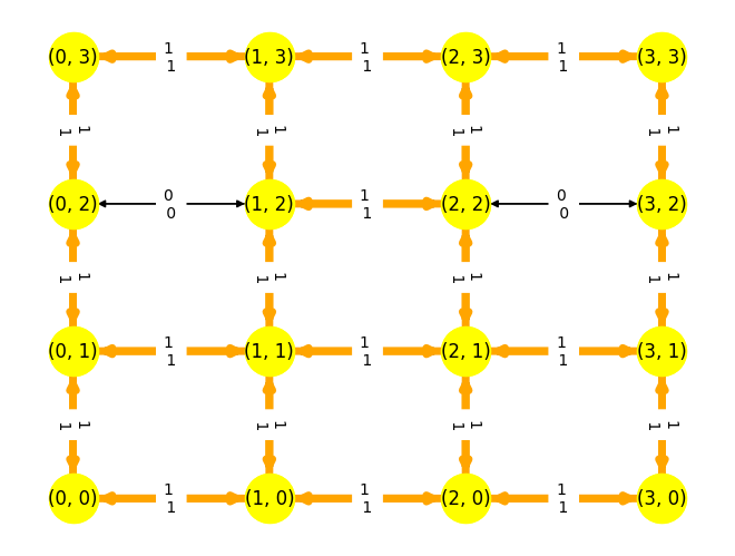

plt.figure()
nx.draw(D, pos=pos, with_labels=True, node_size=1000, node_color="yellow")
edge_labels = {}
edges = []
d = (2,2)
for (i, j) in D.edges():
    if i!=d:
        if  y[i,j,d].X > 0.001:
            edges.append( (i,j) )
            edge_labels[i, j] = f"{int(y[i,j,d].X)} "

nx.draw(D, pos=pos, width=5, edgelist=edges, edge_color="orange", node_size=1000, node_color="yellow")
nx.draw_networkx_edge_labels(D, pos, edge_labels=edge_labels)
plt.show()

パスフロー定式化（入木制約）

集合

• \(\mathcal{V}\): 点集合
• \(\mathcal{E}\): 枝集合
• \(\mathcal{K}\): 品種（発地点，着地点の組）の集合
• \(\mathcal{P}\): パスの集合
• \(\mathcal{P}_{k}\): 品種 \(k\) に対するパスの集合
• \(\mathcal{P}_{ij}\): 枝 \((i,j)\) を通過するパスの集合
• \(\mathcal{D}\): 着地点の集合
• \(\mathcal{E}_p\): パス \(p\) に含まれる枝集合

パラメータ

• \(C_{ij}\): 運搬車の移動（固定）費用
• \(c_p\): パス \(p\) に対する品種の移動（変動）費用の合計
• \(q_p\): パス \(p\) の始点・終点間の需要量
• \(Q\): 運搬車の積載容量

変数

• \(\tau_{ij}\): 運搬車の移動台数を表す整数変数
• \(x_{p}\): パスの使用の有無を表す \(0\)-\(1\) 変数
• \(y_{ij}^d\): 枝 \((i,j)\) が着地 \(d\) へ向かうパス上の枝のとき \(1\) の \(0\)-\(1\) 変数

minimize

\[ \sum_{(i,j) \in \mathcal{E}} (C_{ij} \tau_{ij} + \sum_{p \in \mathcal{P}} c_p x_p) \]

subject to

\[ \sum_{p \in \mathcal{P}_k} x_p = 1 \quad \forall k \in \mathcal{K} \]

\[ \sum_{p \in \mathcal{P}_{ij}} q_p x_{p} \leq Q \tau_{ij} \quad \forall (i,j) \in \mathcal{E} \]

\[ \sum_{(i,j) \in \mathcal{E}} \tau_{ij} - \sum_{(j,i) \in \mathcal{E}} \tau_{ji} = 0 \quad \forall i \in \mathcal{V} \]

\[ \sum_{(i,j) \in \mathcal{E}} y_{ij}^d = 1 \quad \forall d \in \mathcal{D}, \forall i \in \mathcal{V} \]

\[ x_{p} \leq y_{ij}^d \quad \forall (i,j) \in \mathcal{E}_{p}, \forall p \in \mathcal{P}_d, \forall d \in \mathcal{D} \]

\[ y_{ij}^d \in \{0, 1\} \quad \forall d \in \mathcal{D}, \forall (i,j) \in \mathcal{E} \]

\[ \tau_{ij} \in \mathbb{N} \quad \forall (i,j) \in \mathcal{E} \]

plt.figure()
nx.draw(D, pos=pos, with_labels=True, node_size=1000, node_color="yellow")
edge_labels = {}
edges = []
d = (3,3)
for (i, j) in D.edges():
    if i!=d:
        if  y[i,j,d].X > 0.001:
            edges.append( (i,j) )
            edge_labels[i, j] = f"{int(y[i,j,d].X)} "

nx.draw(D, pos=pos, width=5, edgelist=edges, edge_color="orange", node_size=1000, node_color="yellow")
nx.draw_networkx_edge_labels(D, pos, edge_labels=edge_labels)
plt.show()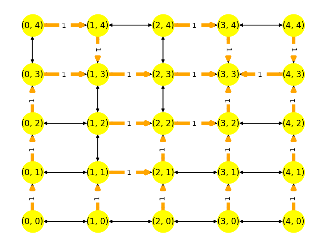

時空間ネットワーク定式化

時空間ネットワークは，地点と時刻の組をノードとしたネットワークであり，移動を表す移動アークとその地点に留まり時刻だけが \(1\) 増加する在庫アークから構成される．

集合

• \(\mathcal{T}\): 時刻（期）の集合

• \(\mathcal{N}_{\mathcal{T}}\): 時空間ネットワークのノード集合

• \(\mathcal{A}_{\mathcal{T}}\): 時空間ネットワークのアーク集合

• \(\mathcal{K}\): 品種（発地点，着地点の組）の集合；品種 \(k\) は発地点 \(o_k\) を時刻 \(e_k\) 以降に出発し， 着地点 \(d_k\) に時刻 \(l_k\) までに到着するものとする．

• \(\mathcal{P}\): パスの集合

• \(\mathcal{P}_{k}\): 品種 \(k\) に対するパスの集合

• \(\mathcal{P}_{ij}\): 枝 \((i,j)\) を通過するパスの集合

• パラメータ

• \(C_{ij}\): 運搬車の移動（固定）費用

• \(c_{ij}^k\): 品種の移動（変動）費用

• \(q_k\): 品種 \(k\) の需要量

• \(Q\): 運搬車の積載容量

変数

• \(\tau_{ij}^{tt'}\): 枝 \(((i,t)(j,t'))\) 上の運搬車の移動台数を表す整数変数
• \(x_{ij}^{ktt'}\): 枝 \(((i,t)(j,t'))\) 上を通過する品種 \(k\) の量を表す実数変数

minimize

\[ \sum_{((i,t),(j,t')) \in \mathcal{A}_{\mathcal{T}}} C_{ij} \tau_{ij}^{tt'} + \sum_{((i,t),(j,t'))} \sum_{k \in \mathcal{K}} c_{ij}^k x_{ij}^{ktt'} \] subject to

\[ \sum_{p \in \mathcal{P}_k} v_p^k = 1 \quad \forall k \in \mathcal{K} \]

\[ \sum_{p \in \mathcal{P}_k} v_p^k = \sum_{(t,t') : ((i,t),(j,t')) \in \mathcal{A}_{\mathcal{T}}} x_{ij}^{ktt'} \quad \forall (i,t) \in \mathcal{N}_{\mathcal{T}}, k \in \mathcal{K} \]

\[ \sum_{((i,t),(j,t')) \in \mathcal{A}_{\mathcal{T}}} x_{ij}^{ktt'} - \sum_{((j,t'),(i,t)) \in \mathcal{A}_{\mathcal{T}}} x_{ji}^{kt't} = \begin{cases} 1 & (i,t) = (o_k, e_k) \\ -1 & (i,t) = (d_k, l_k) \\ 0 & \text{otherwise} \end{cases} \quad \forall (i,t) \in \mathcal{N}_{\mathcal{T}}, \forall k \in \mathcal{K} \]

\[ \sum_{k \in \mathcal{K}} q_k x_{ij}^{ktt'} \leq Q \tau_{ij}^{tt'} \quad \forall ((i,t),(j,t')) \in \mathcal{A}_{\mathcal{T}} \]

\[ \tau_{ij}^{tt'} \in \mathbb{N} \quad \forall ((i,t),(j,t')) \in \mathcal{A}_{\mathcal{T}} \]

\[ v_p^k \in \{0, 1\} \quad \forall k \in \mathcal{K}, p \in \mathcal{P}_k \]

\[ x_{ij}^{ktt'} \in \{0, 1\} \quad \forall ((i,t),(j,t')) \in \mathcal{A}_{\mathcal{T}}, k \in \mathcal{K} \]

flow = {}
for (i, j) in D.edges():
    flow[i, j] = sum(x[i, j, k].X for k in K)
    # for k in K:
    #     if x[i, j, k].X>0.001:
    #         print(i,j,k,x[i, j, k].X)

plt.figure()
nx.draw(D, pos=pos, with_labels=True, node_size=1000, node_color="yellow")
edge_labels = {}
edges = []
for (i, j) in D.edges():
    edge_labels[i, j] = f"{int(flow[i,j])}"
    if  flow[i,j] > 0.001:
        edges.append( (i,j) )
nx.draw(D, pos=pos, width=5, edgelist=edges, edge_color="orange", node_size=1000, node_color="yellow")
nx.draw_networkx_edge_labels(D, pos, edge_labels=edge_labels)
plt.show()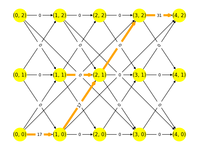

plt.figure()
nx.draw(D, pos=pos, with_labels=True, node_size=1000, node_color="yellow")
edge_labels = {}
edges = []
for (i, j) in D.edges():
    if  y[i,j].X > 0.001:
        edges.append( (i,j) )
    edge_labels[i, j] = f"{int(y[i,j].X)}"

nx.draw(D, pos=pos, width=5, edgelist=edges, edge_color="orange", node_size=1000, node_color="yellow")
nx.draw_networkx_edge_labels(D, pos, edge_labels=edge_labels)
plt.show()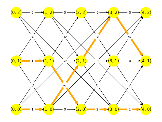

混載ベース定式化

時空間ネットワークを作らずに，品種（荷）の混載だけを考慮した（運搬車の移動経路は考えない）定式化を示す．

集合

• \(\mathcal{V}\): 点集合
• \(\mathcal{E}\): 枝集合
• \(\mathcal{K}\): 品種（発地点，着地点の組）の集合；品種 \(k\) は発地点 \(o_k\) を時刻 \(e_k\) 以降に出発し， 着地点 \(d_k\) に時刻 \(l_k\) までに到着するものとする．
• \(\mathcal{P}\): パスの集合
• \(\mathcal{P}_{k}\): 品種 \(k\) に対するパスの集合
• \(\mathcal{P}_{ij}\): 枝 \((i,j)\) を通過するパスの集合
• \(\Omega_{ij}\): 枝 \((i,j)\) 上での品種の可能な混載の集合； \(\omega \in \Omega_{ij}\) は\(\mathcal{K}\)の部分集合になる．

パラメータ

• \(C_{ij}\): 運搬車の移動（固定）費用
• \(\phi_{\omega}^k\): 品種 \(k\) が混載 \(\omega\) に含まれていか否かを表す \(0\)-\(1\) のパラメータ
• \(s_{\omega}\): 混載 \(\omega\) を運ぶのに必要な運搬車の台数
• \(e_k\): 品種 \(k\) の開始時刻
• \(l_k\): 品種 \(k\) の終了時刻

変数

• \(\tau_{ij}\): 運搬車の移動台数を表す整数変数
• \(\delta_{\omega}\): 混載 \(\omega\) を採用するか否かを表す \(0\)-\(1\) 変数
• \(v_{p}^k\): 品種 \(k\) のパスの使用を表す \(0\)-\(1\) 変数
• \(\gamma_{ij}^k\): 品種\(k\)が枝\((i,j)\)を出発する時刻

minimize

\[ \sum_{(i,j) \in A} C_{ij} \tau_{ij} \]

subject to

各枝・品種に対して，必ず1つの混載を選択しなければならない

\[ \sum_{\omega \in \Omega_{ij}} \phi^k_\omega \delta_\omega = \sum_{p \in \mathcal{P}_{k} } v^k_p \quad \forall (i, j) \in \mathcal{E}, \, k \in \mathcal{K} \]

運搬車の容量制約 \[ \sum_{\omega \in \Omega_{ij}} s_\omega \delta_\omega \leq \tau_{ij} \quad \forall (i, j) \in \mathcal{E} \]

同じ混載になった品種の発時刻が同じでなければならない \[ \gamma^k_{ij} - \gamma^{k'}_{ij} \leq T \left( 1 - \sum_{\omega \in \Omega_{ij}} \phi^k_\omega \phi^{k'}_\omega \delta_\omega \right) \quad \forall (i, j) \in \mathcal{E}, \, k, k' \in \mathcal{K} \]

品種の発時刻の下限制約 \[ \sum_{p \in \mathcal{P}_k} \alpha^{kp}_{ij} v^k_p \leq \gamma^k_{ij} \quad \forall (i, j) \in \mathcal{E}, \, k \in K \]

品種の着時刻の上限制約 \[ \sum_{(i, d_k) \in \mathcal{E}} \left( \gamma^k_{id_k} + \tau_{id_k} \left( \sum_{p \in \mathcal{P}_{k}} v^k_p \right) \right) \leq l_k \quad \forall k \in \mathcal{K} \]

移動開始時刻と移動時間の繋ぎ制約 \[ \sum_{(i,j) \in \mathcal{E}} \left( \gamma^k_{ij} + \tau_{ij} \left( \sum_{p \in \mathcal{P}_k} v^k_p \right) \right) \leq \sum_{(j,i) \in \mathcal{E}} \gamma^k_{ji} \quad \forall j \in \mathcal{N}, \, k \in \mathcal{K} \]

\[ \gamma^k_{ij} \geq 0 \quad \forall k \in K, \, (i, j) \in \mathcal{E} \]

\[ \tau_{ij} \in \mathbb{N} \quad \forall (i, j) \in \mathcal{E} \]

\[ \delta_\omega \in \{0, 1\} \quad \forall \omega \in \Omega_{ij}, \, (i, j) \in \mathcal{E} \]