非線形最適化問題のモデリング

非線形最適化、特に錐最適化のモデリングのコツについて述べる．

ローカルで amplpyを動かす方法

AMPLをインストールしてampl.exeがある場所をEnvironmentで指定する。

from amplpy import AMPL, Environment
env = Environment("/Users/mikiokubo/Documents/ampl/")
ampl = AMPL(env)

Google Colab.で使う場合

ampl_notebook関数で、使うソルバー(modules)とlicense_uuidを設定する（空白でも動く）。

!pip install amplpy
from amplpy import ampl_notebook
ampl = ampl_notebook(
    modules= ["highs","gurobi","cbc","scip","coin","copt","ipopt","couenne","bonmin"]
    license_uuid=None)

錐計画

AMPLでは、二次錐（SOC: Second-Order Cone, 回転二次錐含む）や指数錐（Exponential Cone）といった錐計画問題（Cone Programming）が記述できる。

option solver で錐計画に対応したソルバー（Gurobi、MOSEK、HiGHS）を設定する必要がある。

例：

option solver gurobi;

以下にそれぞれの具体的な例を示す。

二次錐計画問題 (SOCP)

二次錐制約は、以下のような制約である。

\[ \left\{ (x_1, \dots, x_n) \in \mathbb{R}^n ~\mid~ x_1 \ge \sqrt{x_2^2 + x_3^2 + \dots + x_n^2} \right\} \]

この制約は、ベクトル \((x_2,x_3,\cdots,x_n)\) のユークリッド距離（L2ノルム）が、スカラー変数 \(x_1\) によって上から抑えられることを意味する。幾何学的には、原点を頂点とし、\(x_1\) 軸の正の方向に無限に広がる円錐（アイスクリームコーン）のような境界を持つ。幾何学的には「ベクトルの長さがスカラー以下」という意味をもち、制約は凸である。

このため、二次錐計画問題 (Second-order Cone Programming: SOCP) は、効率よく解ける凸最適化問題として扱える。

例として、平面上の複数の点 \((X_1,Y_1), (X_2,Y_2),\cdots,(X_n,Y_n)\) から、距離の総和が最小となる点 \((x,y)\) を求める問題を考える。

\[\min \sum_{i} d_i \quad \text{subject to } \|(x - X_i, y - Y_i)\|_2 \le d_i\]

reset;
# 集合とパラメータ
set POINTS;
param X{POINTS};
param Y{POINTS};

# 変数
var x;
var y;
var d{POINTS} >= 0; # 各点からの距離（上界）

# 目的関数: 距離の総和を最小化
minimize Total_Distance: sum{i in POINTS} d[i];

# 二次錐制約 (in SOC)
subject to Cone_Constraint {i in POINTS}:
    sqrt( (x - X[i])^2 + (y - Y[i])^2 ) <= d[i];

回転二次錐計画問題

上の二次錐を座標平面 \((x_1, x_2)\) 平面において \(\pi/4\) だけ回転させることによって得られるのが、回転二次錐（Rotated Second-Order Cone）である。数学的には、次のような形式を持つ集合として定義される。
\[ \left\{ (u, v, x) \in \mathbb{R}^n ~|~ 2tu \ge x_1^2 + x_2^2 + \dots + x_n^2, \quad u \ge 0, v \ge 0 \right\} \]

例として、\(x_1^2 + x_2^2 \le u \cdot v\) という制約を考える。

reset;
var x1;
var x2;
var u >= 0;
var v >= 0;

# 回転二次錐制約
subject to Rotated_Cone:
    x1^2 + x2^2 <= u*v;

ロバストポートフォリオの定式化

ロバストポートフォリオ（特に期待収益率の不確実性を考慮する場合）を、SOCPとして記述する。

def solve_with_copt():
    ampl = AMPL(env)
    
    # 1. ソルバーをCOPTに設定
    ampl.set_option('solver', 'copt')
    ampl.set_option('copt_options', 'outlev=0')
    ampl.set_option('solver_msg', 0)

    ampl.eval('''
        set ASSETS;
        param mu {ASSETS};
        param R_target;
        param delta;
        var w {ASSETS} >= 0;
        var risk_var >= 0;

        minimize Portfolio_Risk: risk_var;

        subject to Budget:
            sum {i in ASSETS} w[i] = 1;

        subject to Robust_Constraint:
            sum {i in ASSETS} mu[i] * w[i] - delta * risk_var >= R_target;
            
        # SOCP制約
        subject to Cone: sum {i in ASSETS} w[i]^2 <= risk_var^2;
    ''')

    # データのセットアップ
    assets = ['AAPL', 'GOOGL', 'MSFT']
    ampl.get_set('ASSETS').set_values(assets)
    ampl.get_parameter('mu').set_values({'AAPL': 0.12, 'GOOGL': 0.15, 'MSFT': 0.10})
    ampl.get_parameter('R_target').set(0.1)
    ampl.get_parameter('delta').set(0.05)

    # 実行
    ampl.solve()

    # 結果取得
    weights = ampl.get_variable('w').get_values().to_pandas()
    print("Optimization Results with COPT:")
    print(weights)

if __name__ == "__main__":
    solve_with_copt()

COPT 7.2.4:   tech:outlev = 0
Optimization Results with COPT:
          w.val
AAPL   0.314183
GOOGL  0.487061
MSFT   0.198756

感度分析

不確実性パラメータ（不確実性の円の半径） \(\delta\) を変化させたときに、ポートフォリオの資産配分がどのように変化するかの感度分析を行う。この分析を行うことで、「予測が外れるリスクをどれだけ許容するか（ロバスト性の強さ）」によって、投資戦略がどう保守的になっていくかを直感的に理解できる。

import numpy as np
import pandas as pd
import matplotlib.pyplot as plt

def run_robust_sensitivity():
    ampl = AMPL(env)
    ampl.set_option('solver', 'copt')
    ampl.set_option('copt_options', 'outlev=0')
    ampl.set_option('solver_msg', 0)

    # 1. AMPLモデルの定義
    # ここでは期待収益率の不確実性（楕円集合）を考慮したSOCPモデルを使用
    ampl.eval('''
        set ASSETS;
        param mu {ASSETS};
        param R_target;
        param delta; # 不確実性パラメータ
        
        var w {ASSETS} >= 0;
        var risk_var >= 0;

        minimize Portfolio_Risk: risk_var;

        subject to Budget:
            sum {i in ASSETS} w[i] = 1;

        subject to Robust_Constraint:
            sum {i in ASSETS} mu[i] * w[i] - delta * risk_var >= R_target;
            
        subject to Cone: sum {i in ASSETS} w[i]^2 <= risk_var^2;
    ''')

    # 2. サンプルデータの用意
    assets = ['HighRisk_HighReturn', 'Medium_Balanced', 'LowRisk_Safe']
    ampl.get_set('ASSETS').set_values(assets)
    ampl.get_parameter('mu').set_values({
        'HighRisk_HighReturn': 0.20, 
        'Medium_Balanced': 0.12, 
        'LowRisk_Safe': 0.05
    })
    ampl.get_parameter('R_target').set(0.08)

    # 3. デルタ（不確実性）をスイープさせる
    delta_values = np.linspace(0, 0.5, 20)
    results = []

    for d in delta_values:
        ampl.get_parameter('delta').set(d)
        ampl.solve()
        
        # 最適解が得られた場合のみデータを保存
        if ampl.get_value('solve_result') == 'solved':
            w_values = ampl.get_variable('w').get_values().to_dict()
            w_values['delta'] = d
            results.append(w_values)

    # 4. 可視化
    df_results = pd.DataFrame(results).set_index('delta')
    
    plt.figure(figsize=(10, 6))
    df_results.plot.area(stacked=True, alpha=0.7, ax=plt.gca())
    plt.title(r'Robust Portfolio Allocation vs Uncertainty ($\delta$)', fontsize=14)
    plt.xlabel(r'Uncertainty Parameter ($\delta$)', fontsize=12)
    plt.ylabel('Investment Weight', fontsize=12)
    plt.legend(loc='upper right', bbox_to_anchor=(1.3, 1))
    plt.grid(axis='y', linestyle='--', alpha=0.5)
    plt.tight_layout()
    plt.show()

if __name__ == "__main__":
    run_robust_sensitivity()

COPT 7.2.4:   tech:outlev = 0
COPT 7.2.4:   tech:outlev = 0
COPT 7.2.4:   tech:outlev = 0
COPT 7.2.4:   tech:outlev = 0
COPT 7.2.4:   tech:outlev = 0
COPT 7.2.4:   tech:outlev = 0
COPT 7.2.4:   tech:outlev = 0
COPT 7.2.4:   tech:outlev = 0
COPT 7.2.4:   tech:outlev = 0
COPT 7.2.4:   tech:outlev = 0
COPT 7.2.4:   tech:outlev = 0
COPT 7.2.4:   tech:outlev = 0
COPT 7.2.4:   tech:outlev = 0
COPT 7.2.4:   tech:outlev = 0
COPT 7.2.4:   tech:outlev = 0
COPT 7.2.4:   tech:outlev = 0
COPT 7.2.4:   tech:outlev = 0
COPT 7.2.4:   tech:outlev = 0
COPT 7.2.4:   tech:outlev = 0
COPT 7.2.4:   tech:outlev = 0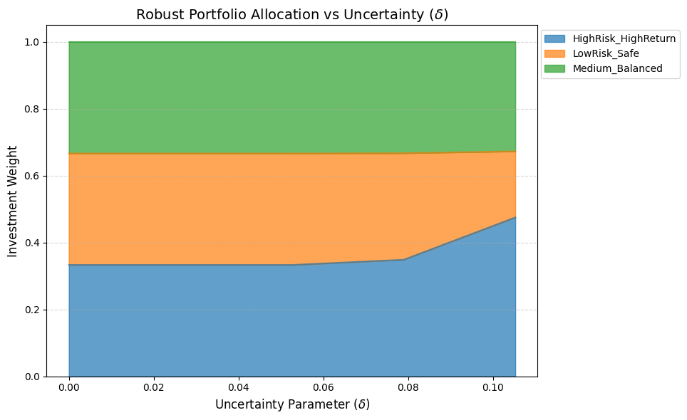

固定費つき生産計画

製品 \(i=1,\dots,n\) について、需要 \(d_i\)、利益 \(p_i\)、固定費 \(f_i\)、二次生産費用 \(a_i > 0\) がある。意思決定変数は、生産量 \(x_i \ge 0\) と、生産するときに \(1\) になる \(y_i \in {0,1}\) である。

モデルは次のように記述できる。

\[ \begin{array}{ll} \text{maximize} & \sum_i p_i x_i - \sum_i f_i y_i - \sum_i a_i x_i^2 \\ \text{subject to} & 0 \le x_i \le d_i y_i \quad \forall i =1,\dots,n \\ & \sum_i c_i x_i \le \text{Cap} \end{array} \]

ここで、\(x_i \le d_i y_i\) により、稼働しない（\(y_i = 0\)）ときは生産量 \(x_i\) が 0 になる。

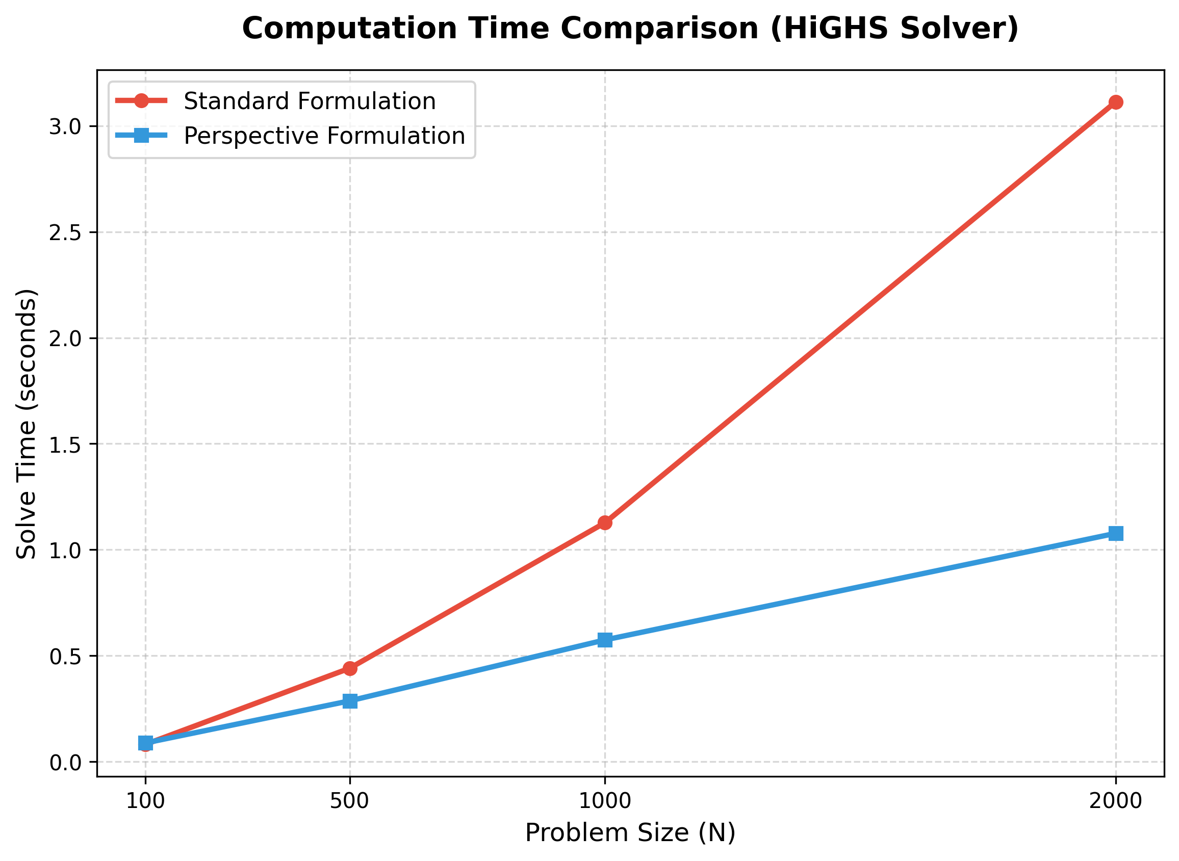
二次費用 \(a_i x_i^2\) は、遠近再定式化 (perspective reformulation) とよばれる手法により、 \(a_i x_i^2 / y_i\) という形の凸緩和に置き換えられ、回転付き二次錐で表すことができる。

各製品について補助変数 \(t_i\) を導入し、

\[t_i \ge a_i \frac{x_i^2}{y_i} \]

を回転付き二次錐で表す。

等価な錐制約のは以下のようになる（この制約はBigMを用いた通常の定式化より強い）。

\[ 2y_i t_i \geq (\sqrt{2a_i}x_i)^2\]

目的関数は \[ \text{maximize} \ \sum_i p_i x_i - \sum_i f_i y_i - \sum_i t_i \] となり、SOCP として解ける。

計算時間の比較結果 (HiGHSソルバー)

普通の定式化（Standard）と遠近定式化（Perspective）のランダムに生成した問題例における計算時間の比較を以下に示す。

from amplpy import AMPL

ampl = AMPL()

model = r"""
set I;

param p {I} >= 0;
param f {I} >= 0;
param a {I} > 0;
param d {I} >= 0;
param c {I} >= 0;
param Cap >= 0;

var x {I} >= 0;
var y {I} binary;
var t {I} >= 0;

maximize Profit:
    sum {i in I} p[i] * x[i]
  - sum {i in I} f[i] * y[i]
  - sum {i in I} t[i];

subject to DemandCap {i in I}:
    x[i] <= d[i] * y[i];

subject to Capacity:
    sum {i in I} c[i] * x[i] <= Cap;

subject to PerspectiveCone {i in I}:
    2 * y[i] * t[i] >= (sqrt(2 * a[i]) * x[i])^2;
"""

ampl.eval(model)

data = {
    "I": ["A", "B"],
    "p": {"A": 10, "B": 12},
    "f": {"A": 30, "B": 40},
    "a": {"A": 0.5, "B": 0.8},
    "d": {"A": 100, "B": 80},
    "c": {"A": 1.0, "B": 1.2},
    "Cap": 120
}

ampl.set["I"] = data["I"]
for i in data["I"]:
    ampl.param["p"][i] = data["p"][i]
    ampl.param["f"][i] = data["f"][i]
    ampl.param["a"][i] = data["a"][i]
    ampl.param["d"][i] = data["d"][i]
    ampl.param["c"][i] = data["c"][i]
ampl.param["Cap"] = data["Cap"]

ampl.option["solver"] = "gurobi"
ampl.solve()

print(ampl.obj["Profit"].value())
for i in ampl.set["I"]:
    print(i, ampl.var["x"][i].value(), ampl.var["y"][i].value(), ampl.var["t"][i].value())

Gurobi 13.0.2:Gurobi 13.0.2: optimal solution; objective 24.99999996
23 simplex iterations
1 branching node
absmipgap=0.00155317, relmipgap=6.21267e-05
24.999999960581384
A 9.99996010670054 1.0 49.99960109246831
B 7.500004309714493 1.0 45.00005173052961

最適潮流問題

非線形最適化の例として最適潮流問題を解く。ソルバーはipopt（coinモジュール）である。

\[ P_i(V, \delta) = P_i^G - P_i^L, \forall i \in N \]

\[ Q_i(V, \delta) = Q_i^G - Q_i^L, \forall i \in N \]

\[ P_i(V, \delta) = V_i \sum_{k=1}^{N}V_k(G_{ik}\cos(\delta_i-\delta_k) + B_{ik}\sin(\delta_i-\delta_k)), \forall i \in N \]

\[ Q_i(V, \delta) = V_i \sum_{k=1}^{N}V_k(G_{ik}\sin(\delta_i-\delta_k) - B_{ik}\cos(\delta_i-\delta_k)), \forall i \in N \]

# data

set N;                              # set of buses in the network
param nL;                           # number of branches in the network
set L within 1..nL cross N cross N; # set of branches in the network
set GEN within N;                   # set of generator buses
set REF within N;                   # set of reference (slack) buses
set PQ within N;                    # set of load buses
set PV within N;                    # set of voltage-controlled buses
set YN :=                           # index of the bus admittance matrix
    setof {i in N} (i,i) union
    setof {(i,k,l) in L} (k,l) union
    setof {(i,k,l) in L} (l,k);

# bus data

param V0     {N}; # initial voltage magnitude
param delta0 {N}; # initial voltage angle
param PL     {N}; # real power load
param QL     {N}; # reactive power load
param g_s    {N}; # shunt conductance
param b_s    {N}; # shunt susceptance


# generator data

param PG {GEN}; # real power generation
param QG {GEN}; # reactive power generation

# branch indexed data

param T    {L}; # initial voltage ratio
param phi  {L}; # initial phase angle
param R    {L}; # branch resistance
param X    {L}; # branch reactance
param g_sh {L}; # shunt conductance
param b_sh {L}; # shunt susceptance

param g {(l,k,m) in L} := R[l,k,m]/(R[l,k,m]^2 + X[l,k,m]^2);  # series conductance
param b {(l,k,m) in L} := -X[l,k,m]/(R[l,k,m]^2 + X[l,k,m]^2); # series susceptance

# bus admittance matrix real part
param G {(i,k) in YN} =
    if (i == k) then (
        g_s[i] +
        sum{(l,i,u) in L} (g[l,i,u] + g_sh[l,i,u]/2)/T[l,i,u]**2 +
        sum{(l,u,i) in L} (g[l,u,i] + g_sh[l,u,i]/2)
    )
    else (
        -sum{(l,i,k) in L} ((
            g[l,i,k]*cos(phi[l,i,k])-b[l,i,k]*sin(phi[l,i,k])
        )/T[l,i,k]) -
        sum{(l,k,i) in L} ((
            g[l,k,i]*cos(phi[l,k,i])+b[l,k,i]*sin(phi[l,k,i])
        )/T[l,k,i])
    );

# bus admittance matrix imaginary part
param B {(i,k) in YN} =
    if (i == k) then (
        b_s[i] +
        sum{(l,i,u) in L} (b[l,i,u] + b_sh[l,i,u]/2)/T[l,i,u]**2 +
        sum{(l,u,i) in L} (b[l,u,i] + b_sh[l,u,i]/2)
    )
    else (
        -sum{(l,i,k) in L} (
            g[l,i,k]*sin(phi[l,i,k])+b[l,i,k]*cos(phi[l,i,k])
        )/T[l,i,k] -
        sum{(l,k,i) in L} (
            -g[l,k,i]*sin(phi[l,k,i])+b[l,k,i]*cos(phi[l,k,i])
        )/T[l,k,i]
    );

# variables
var V     {i in N} := V0[i];     # voltage magnitude
var delta {i in N} := delta0[i]; # voltage angle

# real power injection
var P {i in N} =
    V[i] * sum{(i,k) in YN} V[k] * (
        G[i,k] * cos(delta[i] - delta[k]) +
        B[i,k] * sin(delta[i] - delta[k])
    );

# reactive power injection
var Q {i in N} =
    V[i] * sum{(i,k) in YN} V[k] * (
        G[i,k] * sin(delta[i] - delta[k]) -
        B[i,k] * cos(delta[i] - delta[k])
    );

# constraints

s.t. p_flow {i in (PQ union PV)}:
    P[i] == (if (i in GEN) then PG[i] else 0) - PL[i];

s.t. q_flow {i in PQ}:
    Q[i] == (if (i in GEN) then QG[i] else 0) - QL[i];

s.t. fixed_angles {i in REF}:
    delta[i] == delta0[i];

s.t. fixed_voltages {i in (REF union PV)}:
    V[i] == V0[i];

Overwriting pf.mod

import pandas as pd

df_bus = pd.DataFrame(
    [
        [1, 0.0, 0.0, 0.0, 0.0, 1.0, 1.0],
        [2, 0.0, 0.0, 0.0, 0.3, 0.95, 1.05],
        [3, 0.0, 0.0, 0.05, 0.0, 0.95, 1.05],
        [4, 0.9, 0.4, 0.0, 0.0, 0.95, 1.05],
        [5, 0.239, 0.129, 0.0, 0.0, 0.95, 1.05],
    ],
    columns=["bus", "PL", "QL", "g_s", "b_s", "V_min", "V_max"],
).set_index("bus")

df_branch = pd.DataFrame(
    [
        [1, 1, 2, 0.0, 0.3, 0.0, 0.0, 1.0, 0.0],
        [2, 1, 3, 0.023, 0.145, 0.0, 0.04, 1.0, 0.0],
        [3, 2, 4, 0.006, 0.032, 0.0, 0.01, 1.0, 0.0],
        [4, 3, 4, 0.02, 0.26, 0.0, 0.0, 1.0, -3.0],
        [5, 3, 5, 0.0, 0.32, 0.0, 0.0, 0.98, 0.0],
        [6, 4, 5, 0.0, 0.5, 0.0, 0.0, 1.0, 0.0],
    ],
    columns=["row", "from", "to", "R", "X", "g_sh", "b_sh", "T", "phi"],
).set_index(["row", "from", "to"])

gen = [1, 3, 4]
ref = [1]
pq = [3, 4]
pv = [2, 5]

# print(df_bus)
# print(df_branch)
# data preprocessing

ampl_bus = pd.DataFrame()
cols = ["PL", "QL", "g_s", "b_s"]
for col in cols:
    ampl_bus.loc[:, col] = df_bus.loc[:, col]
ampl_bus["V0"] = 1.0
ampl_bus["delta0"] = 0.0

ampl_branch = pd.DataFrame()
ampl_branch = df_branch.copy()

ampl_gen = pd.DataFrame()
ampl_gen.index = gen
ampl_gen["PG"] = 0.0
ampl_gen["QG"] = 0.0

from math import radians, degrees

# convert degrees to radians
ampl_bus["delta0"] = ampl_bus["delta0"].apply(radians)
ampl_branch["phi"] = ampl_branch["phi"].apply(radians)

print(ampl_bus)
print(ampl_branch)
print(ampl_gen)

        PL     QL   g_s  b_s   V0  delta0
bus                                      
1    0.000  0.000  0.00  0.0  1.0     0.0
2    0.000  0.000  0.00  0.3  1.0     0.0
3    0.000  0.000  0.05  0.0  1.0     0.0
4    0.900  0.400  0.00  0.0  1.0     0.0
5    0.239  0.129  0.00  0.0  1.0     0.0
                 R      X  g_sh  b_sh     T      phi
row from to                                         
1   1    2   0.000  0.300   0.0  0.00  1.00  0.00000
2   1    3   0.023  0.145   0.0  0.04  1.00  0.00000
3   2    4   0.006  0.032   0.0  0.01  1.00  0.00000
4   3    4   0.020  0.260   0.0  0.00  1.00 -0.05236
5   3    5   0.000  0.320   0.0  0.00  0.98  0.00000
6   4    5   0.000  0.500   0.0  0.00  1.00  0.00000
    PG   QG
1  0.0  0.0
3  0.0  0.0
4  0.0  0.0

def pf_run(bus, branch, gen, ref, pq, pv):
    # initialyze AMPL and read the model
    ampl = AMPL(env)
    ampl.read("pf.mod")

    # load the data
    ampl.set_data(bus, "N")
    ampl.param["nL"] = branch.shape[0]
    ampl.set_data(branch, "L")
    ampl.set_data(gen, "GEN")
    ampl.set["REF"] = ref
    ampl.set["PQ"] = pq
    ampl.set["PV"] = pv

    ampl.solve(solver="ipopt")

    solve_result = ampl.get_value("solve_result")
    if solve_result != "solved":
        print("WARNING: solver exited with %s status." % (solve_result,))

    return ampl.get_data("V", "delta").to_pandas(), solve_result


df_res, solver_status = pf_run(ampl_bus, ampl_branch, ampl_gen, ref, pq, pv)

# convert radians back to degrees
df_res["delta"] = df_res["delta"].apply(degrees)

# print results
print("solver status:", solver_status)
print(df_res)

Ipopt 3.12.13: 

******************************************************************************
This program contains Ipopt, a library for large-scale nonlinear optimization.
 Ipopt is released as open source code under the Eclipse Public License (EPL).
         For more information visit http://projects.coin-or.org/Ipopt
******************************************************************************

This is Ipopt version 3.12.13, running with linear solver mumps.
NOTE: Other linear solvers might be more efficient (see Ipopt documentation).

Number of nonzeros in equality constraint Jacobian...:       30
Number of nonzeros in inequality constraint Jacobian.:        0
Number of nonzeros in Lagrangian Hessian.............:       18

Total number of variables............................:        6
                     variables with only lower bounds:        0
                variables with lower and upper bounds:        0
                     variables with only upper bounds:        0
Total number of equality constraints.................:        6
Total number of inequality constraints...............:        0
        inequality constraints with only lower bounds:        0
   inequality constraints with lower and upper bounds:        0
        inequality constraints with only upper bounds:        0

iter    objective    inf_pr   inf_du lg(mu)  ||d||  lg(rg) alpha_du alpha_pr  ls
   0  0.0000000e+00 7.00e-01 0.00e+00  -1.0 0.00e+00    -  0.00e+00 0.00e+00   0
   1  0.0000000e+00 4.87e-02 0.00e+00  -1.7 1.71e-01    -  1.00e+00 1.00e+00h  1
   2  0.0000000e+00 2.17e-04 0.00e+00  -2.5 4.08e-03    -  1.00e+00 1.00e+00h  1
   3  0.0000000e+00 4.11e-09 0.00e+00  -5.7 1.76e-05    -  1.00e+00 1.00e+00h  1

Number of Iterations....: 3

                                   (scaled)                 (unscaled)
Objective...............:   0.0000000000000000e+00    0.0000000000000000e+00
Dual infeasibility......:   0.0000000000000000e+00    0.0000000000000000e+00
Constraint violation....:   4.1074473979318246e-09    4.1074473979318246e-09
Complementarity.........:   0.0000000000000000e+00    0.0000000000000000e+00
Overall NLP error.......:   4.1074473979318246e-09    4.1074473979318246e-09


Number of objective function evaluations             = 4
Number of objective gradient evaluations             = 4
Number of equality constraint evaluations            = 4
Number of inequality constraint evaluations          = 0
Number of equality constraint Jacobian evaluations   = 4
Number of inequality constraint Jacobian evaluations = 0
Number of Lagrangian Hessian evaluations             = 3
Total CPU secs in IPOPT (w/o function evaluations)   =      0.003
Total CPU secs in NLP function evaluations           =      0.000

EXIT: Optimal Solution Found.
 
Ipopt 3.12.13: Optimal Solution Found

suffix ipopt_zU_out OUT;
suffix ipopt_zL_out OUT;
solver status: solved
          V     delta
1  1.000000  0.000000
2  1.000000 -8.657929
3  0.981536 -5.893046
4  0.983056 -9.440548
5  1.000000 -9.950946