!pip install amplpy
from amplpy import ampl_notebook
ampl = ampl_notebook(
    modules=["highs","gurobi","cbc","scip","coin"],
            #coin includes ipopt, couenne, bonmin
license_uuid=None)MPライブラリ
MPライブラリの使用法
![]()
Google Colab.で使う場合
ampl_notebook関数で、使うソルバー(modules)とlicense_uuidを設定する(空白でも動く)。
ローカルで amplpyを動かす方法
AMPLをインストールしてampl.exeがある場所をEnvironmentで指定する。
from amplpy import AMPL, Environment, tools
ampl = AMPL(Environment("/Users/mikiokubo/Documents/ampl/"))
マジックコマンド ampl_eval
マジックコマンド%%ampl_evalをセルの先頭に入れると、そのままAMPLのモデルとコマンドが記述できる。
#%%ampl_eval
reset;
var x1 integer, >= 0;
var x2 integer,  >= 0;
maximize Z: 3*x1 + 2*x2;
subject to Constraint1: 2*x1 + x2 <= 10;
subject to Constraint2: x1==1 or x2 ==5;
option solver gurobi;
solve;

display x1,x2,Z;
Gurobi 12.0.1: optimal solution; objective 19
0 simplex iterations
x1 = 1
x2 = 8
Z = 19
記述したamplモデルは、Pythonのamplインスタンス(グローバル変数)ampl に保管される。
たとえば、evalメソッドで、amplのshow;コマンドを渡すと、モデルの概要が表示される。
ampl.eval("show;")
variables:   x1   x2

constraint:   Constraint1

logical constraint:   Constraint2

objective:   Z
MPサポート
拡張されたMPソルバーインターフェースライブラリは、以下の演算子および式カテゴリーに対する新たなサポートを提供する。
対応しているソルバーは以下の通り。
gurobi
cplex
copt
xpress
mosek
highs
cbc
scip
gcg
MPインターフェイスによって、ソルバーが対応していない場合には、以下を自動的に再定式化する。
条件演算子:
if-then-else,==>,<==,<==>論理演算子:
or,and,not,exists,forall区分的線形関数:
abs,min,max,<<breakpoints; slopes>>計数演算子:
count,atmost,atleast,exactly,numberof関係演算子および比較演算子:
>(=),<(=),!=,alldiff相補性演算子:
complements非線形演算子および関数:
*,/,^,exp,log,sin,cos,tan,sinh,cosh,tanh集合所属演算子:
in
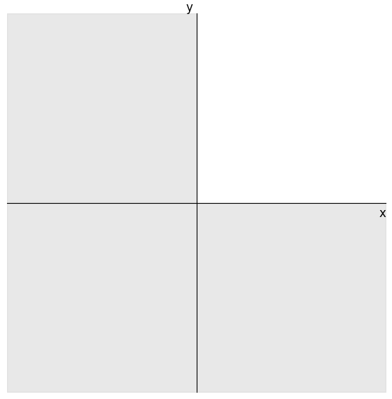
離接制約 or
以下の例では、何れかが正であることを、変数 \(x\) と \(y\) のどちらかが \(0\) 以下である条件として or を用いて記述している。
式の内部表現は solexpand コマンドでみることができる。以下では、セルの先頭のマジックコマンド%%ampl_evalは省略して記述する。
reset;
var x >= -1000, <= 1000;
var y >= -1000, <= 1000;
maximize total: 5 * x + 2 * y;
s.t. only_one_positive: x <= 0 or y <= 0;

option solver highs;
solve;
display x,y;

solexpand only_one_positive;
HiGHS 1.10.0: optimal solution; objective 5000
0 simplex iterations
0 branching nodes
x = 1000
y = 0
subject to only_one_positive:
x <= 0 || y <= 0;
制約only_one_positiveを図示すると以下のようになる。
if then ==>
以下の例では、 何れかが正であることを、もし \(x\) が正なら \(y\) は \(0\) 以下であることを ==> を用いて定義している。
solexpand で内部表現をみると、!(x > 0) || y <= 0 であることが分かる。
reset;
var x >= -1000, <= 1000;
var y >= -1000, <= 1000;
maximize total: 5 * x + 2 * y;
s.t. only_one_positive: x > 0 ==> y <= 0;

option solver highs;
solve;
display x,y;

solexpand only_one_positive;
HiGHS 1.10.0: HiGHS 1.10.0: optimal solution; objective 5000
0 simplex iterations
0 branching nodes
x = 1000
y = 0
subject to only_one_positive:
!(x > 0) || y <= 0;
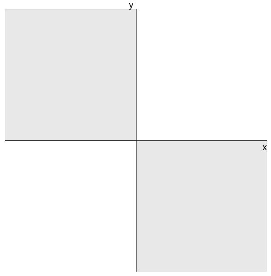
if and only if <==>
以下の例では、 \(x\) と \(y\) のうちの「ちょうど」1つが正であることを、\(x>0\) の必要十分条件が \(y \leq 0\) であると表現し、<==> を用いて記述している。
reset;
var x >= -1000, <= 1000;
var y >= -1000, <= 1000;
minimize total: 5 * x + 2 * y;
s.t. exactly_one_positive: x > 0 <==> y <= 0;

option solver highs;
solve;
display x,y;

solexpand exactly_one_positive;
HiGHS 1.10.0: optimal solution; objective -4999.9998
0 simplex iterations
0 branching nodes
x = -1000
y = 0.0001
subject to exactly_one_positive:
x > 0 <==> y <= 0;
制約exactly_one_positiveを図示すると以下のようになる。
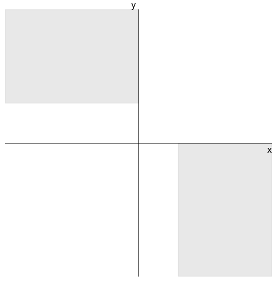
選言標準形
選言標準形 (disjunctive normal form) は、論理式を特定の形式で表現する方法の1つで、 簡単に言うと、「いくつかの(andで結ばれたグループ)が、orで結ばれた形」 である。
以下の例では、\(x\) か \(y\) のいずれかが正で、正の場合には\(3\)以上であることを選言標準形を用いて表現している。
reset;

var x >= -10, <= 10;
var y >= -10, <= 10;
minimize total: 5 * x + 2 * y;
s.t. exactly_one_positive_with_gap:
    (x <= 0 and y >= 3) or (x >= 3 and y <= 0);

option solver highs;
solve;
display x,y;

solexpand exactly_one_positive_with_gap;
HiGHS 1.10.0: optimal solution; objective -44
0 simplex iterations
0 branching nodes
x = -10
y = 3
subject to exactly_one_positive_with_gap:
x <= 0 && y >= 3 || x >= 3 && y <= 0;
この制約を図示すると以下のようになる。
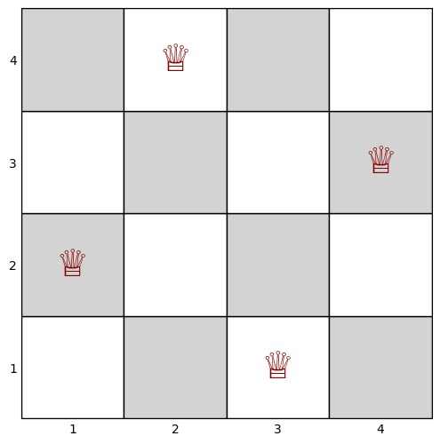
全相異制約 alldiff
8-クイーン問題を例として全相異制約 alldiffを説明する。 alldiff は引数で与えられる変数がすべて異なる値をとることを表す。
8-クイーン問題では、チェス盤にクイーンの駒(縦横斜めに動ける;将棋の飛車と角の動き)を互いに取り合わないように配置する。
各列に置くクイーンの行番号を表す変数 Row が、全て異なり (row_attacks)、Row[j]+jが全て異なり(diag_attacks)、 Row[j]-jが全て異なる(rdiag_attacks)ことで、クイーンが互いに取り合わないことを規定できる。
reset;
param n integer > 0;
var Row {1..n} integer, >= 1, <= n;
s.t. row_attacks: alldiff ({j in 1..n} Row[j]);
s.t. diag_attacks: alldiff ({j in 1..n} Row[j]+j);
s.t. rdiag_attacks: alldiff ({j in 1..n} Row[j]-j);

let n := 8;
option solver gurobi;
solve;
display Row;

solexpand row_attacks;
Gurobi 12.0.1: optimal solution
282 simplex iterations
1 branching node
Objective = find a feasible point.
Row [*] :=
1 7
2 3
3 8
4 2
5 5
6 1
7 6
8 4
;
subject to row_attacks:
alldiff(Row[1], Row[2], Row[3], Row[4], Row[5], Row[6], Row[7], Row[8]);
if .. then ..
以下の例では、ランダムにデータを発生させた施設配置問題において、施設から出る量の合計が正なら、施設の固定費用が必要なことを if .. then ..を 用いて記述している。混合整数最適化問題として記述する場合には、施設を開設するとき \(1\)、それ以外のとき \(0\) になる変数が必要であるが、 if .. then ..を用いても、自動的に \(0\)-\(1\) 変数を追加して求解してくれる。
reset;
# Set up the sets
set I := 1..5;  # potential facility locations
set J := 1..10;  # customers

# Set up the parameters
param f {i in I} = Normal(60, 20);  # fixed costs for each facility
param c {i in I, j in J} = Uniform(10, 30);  # transportation costs from each facility to each customer
param d {j in J} = Uniform(5, 10);  # demand for each customer

# Set up the decision variables
var x {i in I, j in J} >= 0, <= d[j];  # amount of demand for customer j satisfied by facility i

# Set up the objective function
minimize total_cost:
    sum {i in I, j in J} c[i,j]*x[i,j] +
        sum {i in I} if sum {j in J} x[i,j] > 0 then f[i];

# Set up the constraints
subject to demand_constraint {j in J}:
    sum {i in I} x[i,j] = d[j];

option solver highs;
solve;
display x;
HiGHS 1.10.0: optimal solution; objective 1216.446474
7 simplex iterations
1 branching nodes
x [*,*] (tr)
: 1 2 3 4 5 :=
1 0 0 0 0 7.00354
2 0 7.6232 0 0 0
3 9.89917 0 0 0 0
4 0 0 0 0 9.71021
5 0 0 0 6.95342 0
6 0 5.3371 0 0 0
7 0 0 0 0 5.71001
8 0 0 0 8.05193 0
9 9.23089 0 0 0 0
10 0 9.11613 0 0 0
;
不連続な変数の領域
栄養問題を例として、購入量を表す変数 Buyが不連続な領域である場合を考える。
最初の例では、区間[2,5]か区間[7,10]の何れかであることをunion演算子を用いて表現している。
2番目の例では、\(0\) もしくは\(10\)以上\(50\)以下であることを表している。
3番目の例では、\(0\)から\(4\)も整数、もしくは \(9\)から\(13\)の整数、もしくは \(17\)から\(20\)の整数であることを表している。
reset;
model;
set NUTR;
set FOOD;
param cost {FOOD} > 0;
param f_min {FOOD} >= 0;
param f_max {j in FOOD} >= f_min[j];
param n_min {NUTR} >= 0;
param n_max {i in NUTR} >= n_min[i];
param amt {NUTR,FOOD} >= 0;

#union of two intervals
var Buy {FOOD} in interval[2, 5] union interval[7,10]; #最初の例
#var Buy {FOOD} in {0} union interval [10, 50];            #2番目の例
#var Buy {FOOD} in 0..4 union 9..13 union 17..20;         #3番目の例

minimize Total_Cost: sum {j in FOOD} cost[j] * Buy[j];
subject to Diet {i in NUTR}:
n_min[i] <= sum {j in FOOD} amt[i,j] * Buy[j] <= n_max[i];

data;
set NUTR := A B1 B2 C ;
set FOOD := BEEF CHK FISH HAM MCH MTL SPG TUR ;
param:   cost  f_min  f_max :=
BEEF   3.19    0     100
CHK    2.59    0     100
FISH   2.29    0     100
HAM    2.89    0     100
MCH    1.89    0     100
MTL    1.99    0     100
SPG    1.99    0     100
TUR    2.49    0     100 ;
param:   n_min  n_max :=
A      700   10000
C      700   10000
B1     700   10000
B2     700   10000 ;
param amt (tr):
        A    C   B1   B2 :=
BEEF   60   20   10   15
CHK     8    0   20   20
FISH    8   10   15   10
HAM    40   40   35   10
MCH    15   35   15   15
MTL    70   30   15   15
SPG    25   50   25   15
TUR    60   20   15   10 ;

option solver highs;
solve;
display Buy;
HiGHS 1.10.0: optimal solution; objective 101.0133333
7 simplex iterations
1 branching nodes
Buy [*] :=
BEEF 2
CHK 10
FISH 2
HAM 2
MCH 10
MTL 10
SPG 7.33333
TUR 2
;
絶対値 abs
絶対値はabs関数で記述できる。
reset;

var x {1..2} >=-30 <=100;
minimize Objective: abs(x[1]) - 2*abs(x[2]);
s.t. Con1: 3*x[1] - 2*x[2] <=  8;
s.t. Con2: x[1] +   x[2] == 14;

option solver highs;
solve;
display x;

#solexpand Objective;
HiGHS 1.10.0: HiGHS 1.10.0: optimal solution; objective -58
1 simplex iterations
1 branching nodes
x [*] :=
1 -30
2 44
;
最大・最小 min, max
複数の式の最大・最小はmax,min関数を用いて記述できる。 以下では最大値の最小化を行っているので、線形最適化問題のまま求解している。これを最小値の最小化に変えると \(0\)-\(1\)変数が必要になるので、分枝限定法が実行される。 この際、大きな数 (Big M) を用いるので、変数の範囲を明示的に定義しておくことが望ましい(以下の例では\(1000\)以下に設定している)。
reset;
#最大値の最小化(BigMは使わない)
var x {1..2} >=0;
minimize Objective: max( 3 * x[1] + 4 * x[2], 2 * x[1] + 7 * x[2]);
s.t. Con1: x[1] + 2 * x[2] >= 12;
s.t. Con2: 2 * x[1] + x[2] >= 15;

option solver highs;
solve;
display x;
HiGHS 1.10.0: optimal solution; objective 31.2
4 simplex iterations
0 barrier iterations
x [*] :=
1 7.2
2 2.4
;
reset;
#最小値の最小化
#Big Mを使うので、明示的に境界を設定する; gurobiだと設定なしでも解けるが、highsではエラーする、
var x {1..2} >=0, <=1000;
minimize Objective: min( 3 * x[1] + 4 * x[2], 2 * x[1] + 7 * x[2]);
s.t. Con1: x[1] + 2 * x[2] >= 12;
s.t. Con2: 2 * x[1] + x[2] >= 15;

option solver highs;
solve;
display x;
HiGHS 1.10.0: optimal solution; objective 24
8 simplex iterations
1 branching nodes
x [*] :=
1 12
2 0
;
区分的線形関数
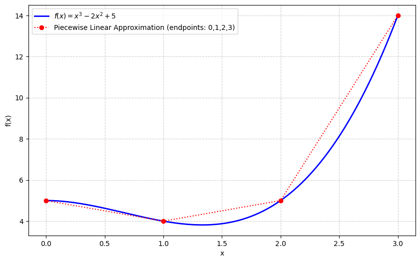
区分的線形関数 (piecewise linear function) は<<端点のリスト;傾きのリスト >>で記述する。
非線形関数 \(x^3-2x^2+5\) を区分的線形近似したときの端点と傾きのリストを準備しておく。 傾きの方が、1つ多いことに注意されたい。
def f(x):
  return x**3-2*x**2+5

def fprime(x):
  return 3*x**2-4*x

xlist=[0,1,2,3]
ylist=list(map(f,xlist))
slope = [fprime(xlist[0])]
for i,x in enumerate(xlist[:-1]):
  slope.append(f(xlist[i+1])-f(x))
slope.append(fprime(xlist[-1]))
print(slope)
[0, -1, 1, 9, 15]以下に、\(x^3-2x^2+5\) と \(0,1,2,3\)を端点とした区分的線形近似関数を示す。
以下のamplのモデルでは、端点のリストはパラメータxlistで、傾きのリストはパラメータslopeで表している。 パラメータは展開した形で代入し、<< >>の後ろには区分的線形関数を適用する変数xを書く。
reset;
var x >=0, <=1000;
param xlist{0..3};
param slope{0..4};
minimize Objective: << {i in 0..3} xlist[i]; {i in 0..4} slope[i] >> x;ampl.param["xlist"] = xlist
ampl.param["slope"] = slopeoption solver highs;
solve;
display x;HiGHS 1.10.0: optimal solution; objective -1
0 simplex iterations
0 barrier iterations
x = 1
数え上げ count, atleast, atmost
輸送問題を例として count, atleast, atmost を解説する。
countは条件を満たす要素の数をカウントする演算子である。 以下の例では、\(600\)以上の輸送量がある経路が少なくとも\(7\)本あること規定している。
subject to Min_Serve:
     count {i in ORIG, j in DEST} (Trans[i,j] >= 600) >= 7;
atmost nは条件を満たす要素の数が高々n個であることを規定する。 以下の例では、\(1000\)以上の輸送量経路が高々\(2\)本があることを表す。
subject to at_most_k:
    atmost 2 {i in ORIG, j in DEST} (Trans[i,j] >= 1000);
atleast nも同様に、条件を満たす要素の数が少なくともn個であることを規定する。
reset;
model;
set ORIG;   # origins
set DEST;   # destinations

param supply {ORIG} >= 0;   # amounts available at origins
param demand {DEST} >= 0;   # amounts required at destinations

   check: sum {i in ORIG} supply[i] = sum {j in DEST} demand[j];

param cost {ORIG,DEST} >= 0;   # shipment costs per unit
var Trans {ORIG,DEST} >= 0;    # units to be shipped

minimize Total_Cost:
   sum {i in ORIG, j in DEST} cost[i,j] * Trans[i,j];

subject to Supply {i in ORIG}:
   sum {j in DEST} Trans[i,j] = supply[i];

subject to Demand {j in DEST}:
   sum {i in ORIG} Trans[i,j] = demand[j];

#少なくとも7本の経路が600以上の輸送量がある
subject to Min_Serve:
     count {i in ORIG, j in DEST} (Trans[i,j] >= 600) >= 7;

#高々2本の経路が1000以上の輸送量がある(等号のtrickで3本のように見えるが、1000-epsilonと解釈)
#subject to at_most_k:
#    atmost 2 {i in ORIG, j in DEST} (Trans[i,j] >= 1000);

data;
param: ORIG:  supply :=  # defines set "ORIG" and param "supply"
        GARY   1400
        CLEV   2600
        PITT   2900 ;

param: DEST:  demand :=  # defines "DEST" and "demand"
        FRA     900
        DET    1200
        LAN     600
        WIN     400
        STL    1700
        FRE    1100
        LAF    1000 ;

param cost:
         FRA  DET  LAN  WIN  STL  FRE  LAF :=
   GARY   39   14   11   14   16   82    8
   CLEV   27    9   12    9   26   95   17
   PITT   24   14   17   13   28   99   20 ;

option solver gurobi; #highsだと解けない
solve;
display Trans;
Gurobi 12.0.1: tech:writegraph = model.jsonl
Gurobi 12.0.1: optimal solution; objective 197000
26 simplex iterations
1 branching node
Trans [*,*] (tr)
: CLEV GARY PITT :=
DET 1200 0 0
FRA 0 0 900
FRE 0 1100 0
LAF 0 300 700
LAN 600 0 0
STL 600 0 1100
WIN 200 0 200
;
非線形関数
以下の非線形関数をそのまま記述することができる。
- log (expr), log10 (expr)
- exp (expr)
- sin (expr), cos (expr), tan (expr), asin (expr), acos (expr), atan (expr)
- sinh (expr), cosh (expr), tanh (expr), asinh (expr), acosh (expr), atanh (expr)
- expr1 ^ expr2
ソルバーが対応可能な場合はそのまま、非対応の場合には区分的線形関数に近似する。
例として、3次関数 \(x^3-2x^2+5\) の最小化を行う。区分的線形近似のためには、変数 \(x\) の範囲を明示的に定義しておく必要がある。
自動的に区分的線形近似が行われ、最適解\(4/3=1.33\cdots\)に近い解が得られることが確認できる。
reset;
model;
var x >=0, <=3;
minimize Objective: x^3-2*x^2+5;
option solver gorobi; #highsだと間違える;gurobiかscipもしくは非線形最適化ソルバー(knitro, ipopt)を用いる
solve;
display x;
Cannot find "gorobi"
x = 0