NeuralProphetによる時系列データの予測

需要予測パッケージ NeuralProphet を紹介する．

NeuralProphetとは

NeuralProphet は需要予測のためのパッケージである．

Bayes推論に基づく予測パッケージ prophet と機械（深層）学習の橋渡しのために新たに開発されたもので、深層学習パッケージ PyTorch を用いている。

vega_datasetsのデータを用いるので，インストールしておく．

# Google Colabで実行する場合は以下を実行しておく。
# !pip uninstall -y torch notebook notebook_shim tensorflow tensorflow-datasets prophet torchaudio torchdata torchtext torchvision
# インストールされていない場合には、以下を生かす。
# !pip install -U neuralprophet
# !pip install -U vega_datasets
# !pip install -U ipywidgets

諸パッケージのインポート

NeuralProphetで予測するために必要なパッケージをインポートしておく．

import pandas as pd
from neuralprophet import NeuralProphet, set_log_level

# エラー以外はログメッセージを抑制
set_log_level("ERROR")

from vega_datasets import data
import plotly.express as px
import plotly

NeuralProphetの基本

NeuralProphetをPythonから呼び出して使う方法は，機械学習パッケージscikit-learnと同じである。

1. NeuralProphetクラスのインスタンスmodelを生成
2. fitメソッドで学習（引数はデータフレーム、返値は評価尺度）
3. predictメソッドで予測（引数は予測したい期間を含んだデータフレーム）

例題：Wikiアクセス数

例としてアメリカンフットボールプレーヤのPayton ManningのWikiアクセス数のデータを用いる。

df = pd.read_csv("http://logopt.com/data/peyton_manning.csv")
df.head()

	ds	y
0	2007-12-10	9.590761
1	2007-12-11	8.519590
2	2007-12-12	8.183677
3	2007-12-13	8.072467
4	2007-12-14	7.893572

Prophetモデルのインスタンスを生成し，fitメソッドで学習（パラメータの最適化）を行う．fitメソッドに渡すのは，上で作成したデータフレームである．このとき、ds(datestamp)列に日付（時刻）を、y列に予測したい数値を入れておく必要がある （この例題では，あらかじめそのように変更されている）．

model = NeuralProphet()
metrics = model.fit(df)

WARNING - (py.warnings._showwarnmsg) - /Users/mikiokubo/Library/Caches/pypoetry/virtualenvs/analytics2-0ZiTWol9-py3.9/lib/python3.9/site-packages/pytorch_lightning/trainer/setup.py:201: UserWarning:

MPS available but not used. Set `accelerator` and `devices` using `Trainer(accelerator='mps', devices=1)`.

make_future_dataframeメソッドで未来の時刻を表すデータフレームを生成する。 既定値では予測で用いた過去の時刻も含まないので、n_historic_predictions引数をTrueにして、過去の時刻も入れる。 引数は予測をしたい期間数periodsであり，ここでは、１年後（365日分）まで予測することにする。

df_future = model.make_future_dataframe(df, n_historic_predictions=True, periods=365)
forecast = model.predict(df_future)
model.set_plotting_backend("matplotlib") #matplotlibで描画する（既定値はplotly）
model.plot(forecast)

predict メソッドに予測したい時刻を含んだデータフレームfuture を渡すと、予測値を入れたデータフレームforecastを返す。

forecast.tail()

	ds	y	yhat1	trend	season_yearly	season_weekly
3265	2017-01-15	NaN	8.216602	7.137280	1.036658	0.042665
3266	2017-01-16	NaN	8.550267	7.136175	1.049828	0.364264
3267	2017-01-17	NaN	8.316690	7.135070	1.060175	0.121446
3268	2017-01-18	NaN	8.133187	7.133965	1.067564	-0.068342
3269	2017-01-19	NaN	8.133450	7.132861	1.071885	-0.071296

一般化加法モデル

NeuralProphetにおける予測は一般化加法モデルを用いて行われる． これは，傾向変動，季節変動，イベント情報などの様々な因子の和として予測を行う方法である．

\[ y_t =g_t + s_t + h_t + f_t + a_t + \ell_t + \epsilon_t \]

• \(y_t\) : 予測値
• \(g_t\) : 傾向変動(trend)；傾向変化点ありの区分的線形（アフィン）関数
• \(s_t\) : 季節変動；年次，週次，日次の季節変動をsin, cosの組み合わせ（フーリエ級数）で表現
• \(h_t\) : 休日などのイベント項
• \(f_t\): 外生変数に対する回帰項
• \(a_t\): 自己回帰項（時間遅れ（ラグ）を指定する）
• \(\ell_t\): 時間遅れ（ラグ）付きの外生変数に対する回帰項
• \(\epsilon_t\) : 誤差項

因子ごとに予測値の描画を行うには，plot_componentsメソッドを用いる．既定では，以下のように，上から順に傾向変動，年次の季節変動、週次の季節変動が描画される．また，傾向変動の図（一番上）には，予測の誤差範囲が示される．季節変動の誤差範囲を得る方法については，後述する．

model.plot_components(forecast)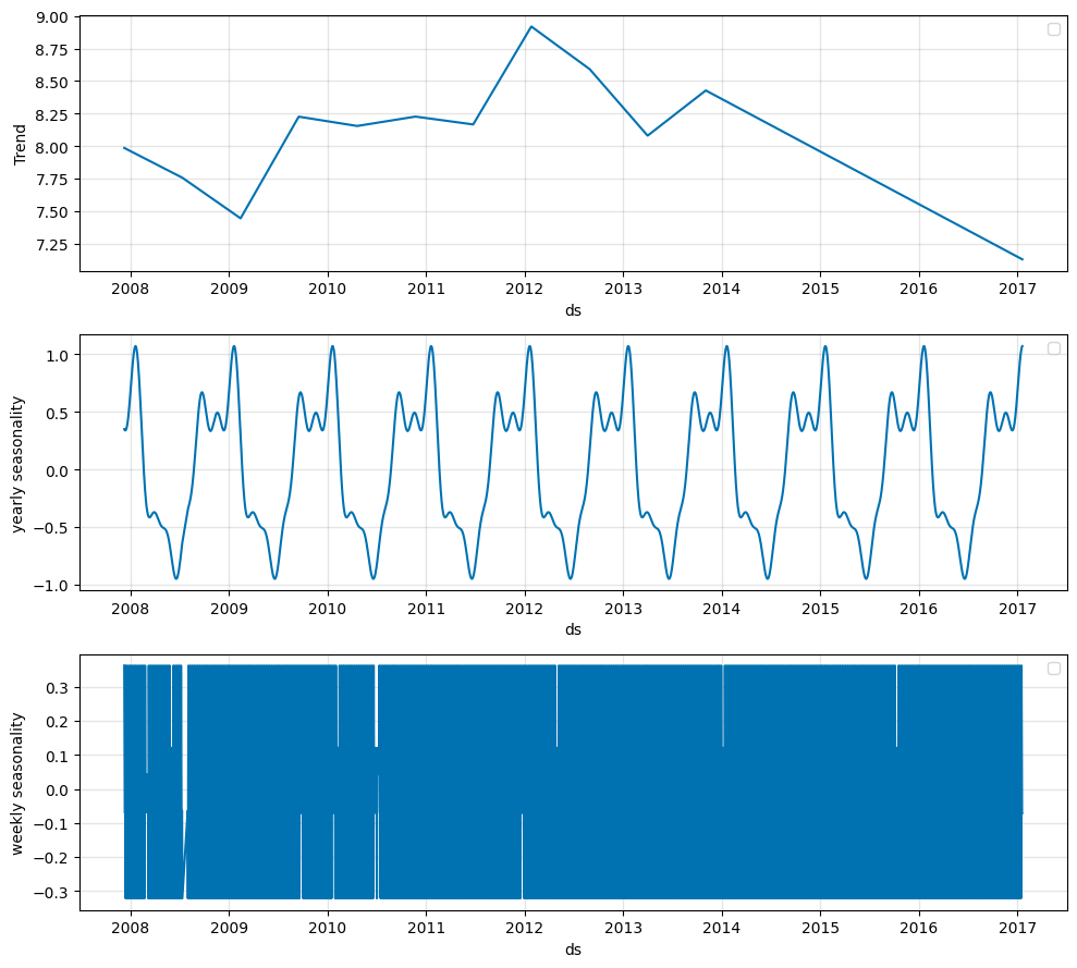

対話形式に，拡大縮小や範囲指定ができる動的な図も，Plotlyライブラリを用いて得ることができる．

model.set_plotting_backend("plotly") 
fig = model.plot(forecast)
#plotly.offline.plot(fig);

例題： \(CO_2\) 排出量のデータ

データライブラリから二酸化炭素排出量のデータを読み込み，Plotly Expressで描画する．

co2 = data.co2_concentration()
co2.head()

	Date	CO2
0	1958-03-01	315.70
1	1958-04-01	317.46
2	1958-05-01	317.51
3	1958-07-01	315.86
4	1958-08-01	314.93

fig = px.line(co2,x="Date",y="CO2")
#plotly.offline.plot(fig);

列名の変更には，データフレームのrenameメソッドを用いる．引数はcolumnsで，元の列名をキーとし，変更後の列名を値とした辞書を与える．また，元のデータフレームに上書きするために，inplace引数をTrueに設定しておく．

co2.rename(columns={"Date":"ds","CO2":"y"},inplace=True)
co2.head()

	ds	y
0	1958-03-01	315.70
1	1958-04-01	317.46
2	1958-05-01	317.51
3	1958-07-01	315.86
4	1958-08-01	314.93

make_future_dataframeメソッドで未来の時刻を表すデータフレームを生成する。既定値では、（予測で用いた）過去の時刻も含む。 ここでは、200ヶ月先まで予測することにする。

そのために，引数 periods を200に設定しておく

predict メソッドに予測したい時刻を含んだデータフレームfuture を渡すと、予測値を入れたデータフレームforecastを返す。

最後にplotメソッドで表示する．

model = NeuralProphet()
metrics = model.fit(co2)
future = model.make_future_dataframe(co2, n_historic_predictions=True, periods=200)
forecast = model.predict(future)
model.set_plotting_backend("plotly")
model.plot(forecast)

WARNING - (py.warnings._showwarnmsg) - /Users/mikiokubo/Library/Caches/pypoetry/virtualenvs/analytics2-0ZiTWol9-py3.9/lib/python3.9/site-packages/pytorch_lightning/trainer/setup.py:201: UserWarning:

MPS available but not used. Set `accelerator` and `devices` using `Trainer(accelerator='mps', devices=1)`.

予測は一般化加法モデルを用いて行われる．

これは，傾向変動，季節変動，イベント情報などの様々な因子の和として予測を行う方法である．

上に表示されているように，週次と日次の季節変動は無視され，年次の季節変動のみ考慮して予測している．

因子ごとに予測値の描画を行うには，plot_componentsメソッドを用いる．既定では，以下のように，上から順に傾向変動，年次の季節変動が描画される．

model.plot_components(forecast)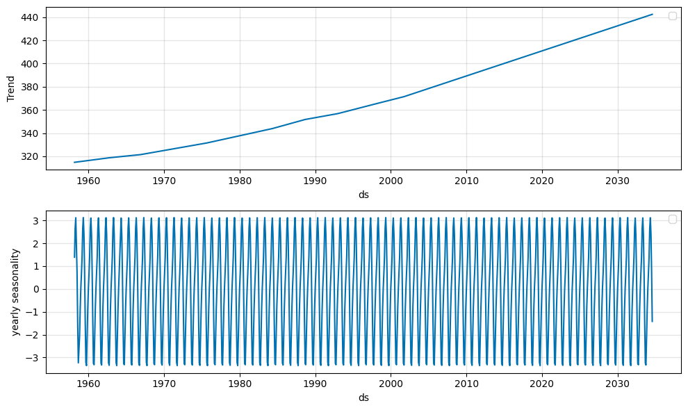

例題：航空機乗客数のデータ

Prophetの既定値では季節変動は加法的モデルであるが、問題によっては乗法的季節変動の方が良い場合もある。 例として、航空機の乗客数を予測してみよう。最初に既定値の加法的季節変動モデルで予測し，次いで乗法的モデルで予測する．

passengers = pd.read_csv("http://logopt.com/data/AirPassengers.csv")
passengers.head()

	Month	#Passengers
0	1949-01	112
1	1949-02	118
2	1949-03	132
3	1949-04	129
4	1949-05	121

fig = px.line(passengers,x="Month",y="#Passengers")
#plotly.offline.plot(fig);

passengers.rename(inplace=True,columns={"Month":"ds","#Passengers":"y"})
passengers.head()

	ds	y
0	1949-01	112
1	1949-02	118
2	1949-03	132
3	1949-04	129
4	1949-05	121

季節変動を乗法的に変更するには， モデルの seasonality_mode 引数を乗法的を表す multiplicative に設定する．

また、モデルを作成するときに、引数quantilesで不確実性の幅を表示するようにする。以下では、5%と95%の幅を表示させている。

model = NeuralProphet(quantiles=[0.05, 0.95])
metrics = model.fit(passengers)
future = model.make_future_dataframe(passengers, periods=20, n_historic_predictions=True)
forecast = model.predict(future)
model.set_plotting_backend("plotly")
model.plot(forecast)

WARNING - (py.warnings._showwarnmsg) - /Users/mikiokubo/Library/Caches/pypoetry/virtualenvs/analytics2-0ZiTWol9-py3.9/lib/python3.9/site-packages/pytorch_lightning/trainer/setup.py:201: UserWarning:

MPS available but not used. Set `accelerator` and `devices` using `Trainer(accelerator='mps', devices=1)`.

model = NeuralProphet(quantiles=[0.05, 0.95], seasonality_mode="multiplicative")
metrics = model.fit(passengers)
future = model.make_future_dataframe(passengers, periods=20, n_historic_predictions=True)
forecast = model.predict(future)
model.set_plotting_backend("plotly")
model.plot(forecast)

WARNING - (py.warnings._showwarnmsg) - /Users/mikiokubo/Library/Caches/pypoetry/virtualenvs/analytics2-0ZiTWol9-py3.9/lib/python3.9/site-packages/pytorch_lightning/trainer/setup.py:201: UserWarning:

MPS available but not used. Set `accelerator` and `devices` using `Trainer(accelerator='mps', devices=1)`.

結果から，乗法的季節変動の方が，良い予測になっていることが確認できる．

問題（小売りの需要データ）

以下の，小売りの需要データを描画し，予測を行え． ただし，モデルは乗法的季節変動で，月次で予測せよ．

retail = pd.read_csv(`http://logopt.com/data/retail_sales.csv`)
retail.head()

	ds	y
0	1992-01-01	146376
1	1992-02-01	147079
2	1992-03-01	159336
3	1992-04-01	163669
4	1992-05-01	170068

例題： 1時間ごとの気温データ

ここではシアトルの気温の予測を行う．

climate = data.seattle_temps()
climate.head()

	date	temp
0	2010-01-01 00:00:00	39.4
1	2010-01-01 01:00:00	39.2
2	2010-01-01 02:00:00	39.0
3	2010-01-01 03:00:00	38.9
4	2010-01-01 04:00:00	38.8

このデータは， date 列に日付と1時間ごとの時刻が， temp 列に気温データが入っている．

NeuralProphetは， 日別でないデータも扱うことができる。 date列のデータ形式は、日付を表すYYYY-MM-DDの後に時刻を表すHH:MM:SSが追加されている。 未来の時刻を表すデータフレームは、make_future_dataframeメソッドで生成する。

climate["Date"] = pd.to_datetime(climate.date)

climate.rename(columns={"Date":"ds","temp":"y"},inplace=True)

climate = climate[["ds","y"]] #余分な列を削除する

model = NeuralProphet(daily_seasonality=True)
metrics = model.fit(climate)
future = model.make_future_dataframe(climate, periods=200, n_historic_predictions=True)
forecast = model.predict(future)
model.set_plotting_backend("plotly")
model.plot(forecast)

WARNING - (py.warnings._showwarnmsg) - /Users/mikiokubo/Library/Caches/pypoetry/virtualenvs/analytics2-0ZiTWol9-py3.9/lib/python3.9/site-packages/pytorch_lightning/trainer/setup.py:201: UserWarning:

MPS available but not used. Set `accelerator` and `devices` using `Trainer(accelerator='mps', devices=1)`.

因子ごとに予測値を描画すると，傾向変動と週次の季節変動の他に，日次の季節変動（1日の気温の変化）も出力される．

model.plot_components(forecast)

問題（サンフランシスコの気温データ）

以下のサンフランシスコの気温データを描画し，時間単位で予測を行え．

sf = data.sf_temps()
sf.head()

	temp	date
0	47.8	2010-01-01 00:00:00
1	47.4	2010-01-01 01:00:00
2	46.9	2010-01-01 02:00:00
3	46.5	2010-01-01 03:00:00
4	46.0	2010-01-01 04:00:00

傾向変化点

「上昇トレンドの株価が，下降トレンドに移った」というニュースをよく耳にするだろう．このように，傾向変動は，時々変化すると仮定した方が自然なのだ．NeuralProphetでは，これを傾向変化点として処理する．再び，Peyton Manningのデータを使う．

傾向変化点の数はn_changepointsで指定する。既定値は \(10\) である。以下では、傾向変化点を \(5\) に設定する。

df = pd.read_csv("http://logopt.com/data/peyton_manning.csv")
model = NeuralProphet(n_changepoints=5)
model.fit(df)
future = model.make_future_dataframe(df, periods=365, n_historic_predictions=True)
forecast = model.predict(future)
model.plot(forecast)

WARNING - (py.warnings._showwarnmsg) - /Users/mikiokubo/Library/Caches/pypoetry/virtualenvs/analytics2-0ZiTWol9-py3.9/lib/python3.9/site-packages/pytorch_lightning/trainer/setup.py:201: UserWarning: MPS available but not used. Set `accelerator` and `devices` using `Trainer(accelerator='mps', devices=1)`.
  rank_zero_warn(

model.plot_components(forecast)

傾向変化点のリストをchangepoints引数で与えることもできる。以下の例では、1つの日だけで変化するように設定している。

model = NeuralProphet(changepoints=["2014-01-01"])
model.fit(df)
future = model.make_future_dataframe(df, periods=365, n_historic_predictions=True)
forecast = model.predict(future)
model.plot(forecast)

WARNING - (py.warnings._showwarnmsg) - /Users/mikiokubo/Library/Caches/pypoetry/virtualenvs/analytics2-0ZiTWol9-py3.9/lib/python3.9/site-packages/pytorch_lightning/trainer/setup.py:201: UserWarning:

MPS available but not used. Set `accelerator` and `devices` using `Trainer(accelerator='mps', devices=1)`.

model.plot_components(forecast)

例題 SP500データ

株価の予測を行う．

傾向変化点の候補は自動的に設定される。既定値では時系列の最初の80%の部分に均等に設定される。これは、モデルのchangepoint_range引数で設定する． この例では，期間の終わりで変化点を設定したいので，0.95に変更する．

年次の季節変動の変化の度合いは、yearly_seasonality（既定値は \(10\)) で制御できる。この例では，このパラメータを \(5\) に変更することによって年間の季節変動を抑制して予測を行う．

sp500 = data.sp500()
sp500.tail()

	date	price
118	2009-11-01	1095.63
119	2009-12-01	1115.10
120	2010-01-01	1073.87
121	2010-02-01	1104.49
122	2010-03-01	1140.45

sp500.rename(inplace=True,columns={"date":"ds","price":"y"})

model = NeuralProphet(changepoints_range=0.95, yearly_seasonality=5)
model.fit(sp500)
future = model.make_future_dataframe(sp500, periods=20, n_historic_predictions=True)
forecast = model.predict(future)
model.plot(forecast)

WARNING - (py.warnings._showwarnmsg) - /Users/mikiokubo/Library/Caches/pypoetry/virtualenvs/analytics2-0ZiTWol9-py3.9/lib/python3.9/site-packages/pytorch_lightning/trainer/setup.py:201: UserWarning:

MPS available but not used. Set `accelerator` and `devices` using `Trainer(accelerator='mps', devices=1)`.

model.plot_components(forecast)

例題： 個別銘柄の株価の予測

stocksデータでは，symbol列に企業コードが入っている．

• AAPL アップル
• AMZN アマゾン
• IBM IBM
• GOOG グーグル
• MSFT マイクロソフト

まずは可視化を行う。

stocks = data.stocks()
stocks.tail()

	symbol	date	price
555	AAPL	2009-11-01	199.91
556	AAPL	2009-12-01	210.73
557	AAPL	2010-01-01	192.06
558	AAPL	2010-02-01	204.62
559	AAPL	2010-03-01	223.02

fig = px.line(stocks,x="date",y="price",color="symbol")
#plotly.offline.plot(fig);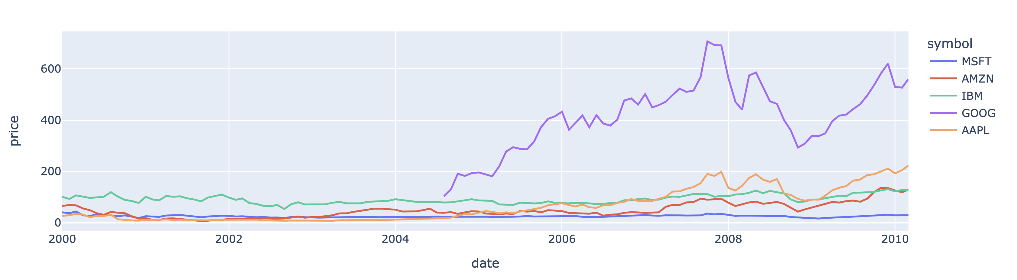

以下では，マイクロソフトの株価を予測してみる．

msft = stocks[stocks.symbol == "MSFT"]
msft.head()

	symbol	date	price
0	MSFT	2000-01-01	39.81
1	MSFT	2000-02-01	36.35
2	MSFT	2000-03-01	43.22
3	MSFT	2000-04-01	28.37
4	MSFT	2000-05-01	25.45

msft = msft.rename(columns={"date":"ds","price":"y"})
msft = msft[["ds","y"]]
msft.head()

	ds	y
0	2000-01-01	39.81
1	2000-02-01	36.35
2	2000-03-01	43.22
3	2000-04-01	28.37
4	2000-05-01	25.45

model = NeuralProphet(changepoints_range=0.95,yearly_seasonality=5)
model.fit(msft)
future = model.make_future_dataframe(msft, periods=20, n_historic_predictions=True)
forecast = model.predict(future)
model.plot(forecast)

WARNING - (py.warnings._showwarnmsg) - /Users/mikiokubo/Library/Caches/pypoetry/virtualenvs/analytics2-0ZiTWol9-py3.9/lib/python3.9/site-packages/pytorch_lightning/trainer/setup.py:201: UserWarning:

MPS available but not used. Set `accelerator` and `devices` using `Trainer(accelerator='mps', devices=1)`.

#model.plot_components(forecast)
model.plot_parameters(forecast)

問題（株価）

上の株価データのマイクロソフト以外の銘柄を1つ選択し，予測を行え．

stocks = data.stocks()
stocks.head()

	symbol	date	price
0	MSFT	2000-01-01	39.81
1	MSFT	2000-02-01	36.35
2	MSFT	2000-03-01	43.22
3	MSFT	2000-04-01	28.37
4	MSFT	2000-05-01	25.45

発展編

以下では，NeuralProphetの高度な使用法を解説する．

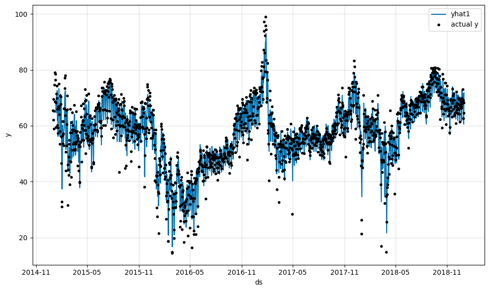
自己回帰による予測

以下の例は、スペインの4年間のエネルギー価格である。 直近の \(p\) 日前までのデータの重み付きの和の項を追加するのが、自己回帰モデルである。 \(p\) を表すn_legs引数を設定すると、自己回帰項が追加される。

df = pd.read_csv("https://github.com/ourownstory/neuralprophet-data/raw/main/kaggle-energy/datasets/tutorial01.csv")
df.head()

	ds	y
0	2014-12-31	65.41
1	2015-01-01	62.09
2	2015-01-02	69.44
3	2015-01-03	65.22
4	2015-01-04	58.91

model = NeuralProphet(
    yearly_seasonality=True,
    weekly_seasonality=True,
    daily_seasonality=True,
    n_lags=10
)
model.set_plotting_backend("matplotlib")
metrics = model.fit(df)
forecast = model.predict(df)
model.plot(forecast)

WARNING - (py.warnings._showwarnmsg) - /Users/mikiokubo/Library/Caches/pypoetry/virtualenvs/analytics2-0ZiTWol9-py3.9/lib/python3.9/site-packages/pytorch_lightning/trainer/setup.py:201: UserWarning:

MPS available but not used. Set `accelerator` and `devices` using `Trainer(accelerator='mps', devices=1)`.

model.plot_parameters()

休日（特別なイベント）を考慮した予測

休日や特別なイベントをモデルに追加することを考える。

モデルインスタンスのadd_country_holidaysメソッドを用いて，各国（州）の休日データを追加することができる。 引数は python-holidays にある文字列で、 たとえば米国の場合にはUS、スペインの場合にはESを指定する。

df = pd.read_csv("https://github.com/ourownstory/neuralprophet-data/raw/main/kaggle-energy/datasets/tutorial01.csv")
df.head()

	ds	y
0	2014-12-31	65.41
1	2015-01-01	62.09
2	2015-01-02	69.44
3	2015-01-03	65.22
4	2015-01-04	58.91

model = NeuralProphet()
model.set_plotting_backend("matplotlib")
model = model.add_country_holidays("US")
metrics = model.fit(df)
forecast = model.predict(df)
model.plot(forecast)

model.plot_components(forecast)

悪天候(extreme_weather)を表すデータフレームを与えることによって、特別なイベントを考慮した予測を行うことができる。 データフレームはeventとdsの列をもち、それをadd_eventsメソッドで追加する。 その後、create_df_with_eventsでイベントが追加されたデータフレームを生成する。

df_events = pd.DataFrame(
    {
        "event": "extreme_weather",
        "ds": pd.to_datetime(
            [
                "2018-11-23",
                "2018-11-17",
                "2018-10-28",
                "2018-10-18",
                "2018-10-14",
            ]
        ),
    }
)
df_events.head()

	event	ds
0	extreme_weather	2018-11-23
1	extreme_weather	2018-11-17
2	extreme_weather	2018-10-28
3	extreme_weather	2018-10-18
4	extreme_weather	2018-10-14

model = NeuralProphet()
model.set_plotting_backend("matplotlib")
model.add_events("extreme_weather")
df_all = model.create_df_with_events(df, df_events)
df_all.head()

	ds	y	extreme_weather
0	2014-12-31	65.41	0.0
1	2015-01-01	62.09	0.0
2	2015-01-02	69.44	0.0
3	2015-01-03	65.22	0.0
4	2015-01-04	58.91	0.0

metrics = model.fit(df_all)
forecast = model.predict(df_all)
model.plot(forecast)

外生変数の追加

外生変数である気温temperatureを利用してエネルギー価格の予測を行う。

ここでは、\(q\) 日前までの気温がエネルギー価格に影響を与える時間遅れ（ラグ）モデルを用いる。 モデルインスタンスのaddd_lagged_regressorメソッドを用いる。 引数は列名もしくは列名のリストである。時間遅れのパラメータ \(q\) は引数n_lagsで与える。

また、未来の気温が既知であると仮定した場合には、気温を外生変数とした回帰項を追加する。 これには、モデルインスタンスの add_future_regressorを用いる。 引数は列名もしくは列名のリストである。

df = pd.read_csv("https://github.com/ourownstory/neuralprophet-data/raw/main/kaggle-energy/datasets/tutorial04.csv")
df.head()

	ds	y	temperature
0	2015-01-01	64.92	277.00
1	2015-01-02	58.46	277.95
2	2015-01-03	63.35	278.83
3	2015-01-04	50.54	279.64
4	2015-01-05	64.89	279.05

model = NeuralProphet(
    yearly_seasonality=True,
    weekly_seasonality=True,
    daily_seasonality=True,
    n_lags=10
)
model.set_plotting_backend("matplotlib")
#model.add_lagged_regressor("temperature", n_lags=5)
model.add_future_regressor("temperature")
metrics = model.fit(df)
forecast = model.predict(df)
model.plot(forecast)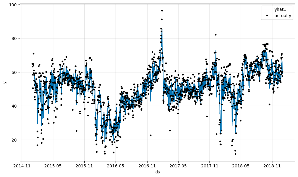

model.plot_parameters()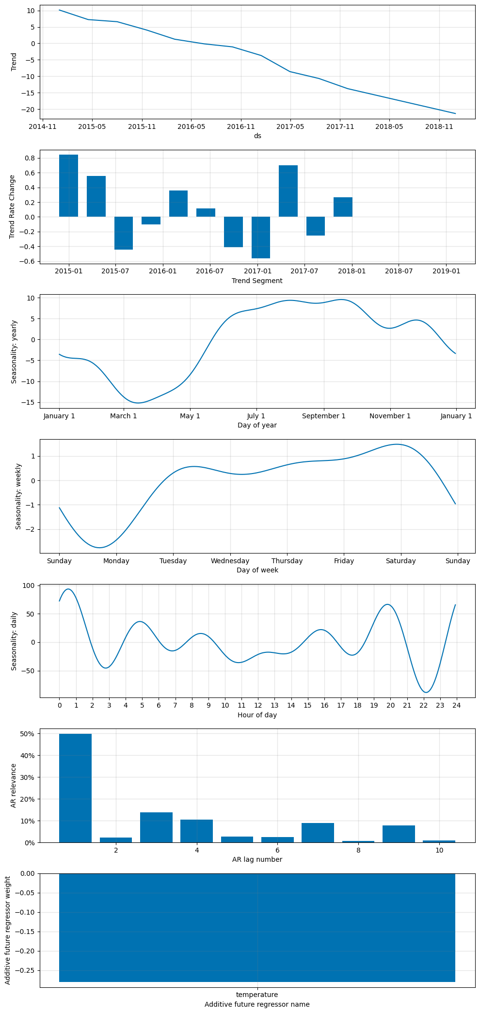

ユーザーが設定した季節変動

Prophetでは既定値の年次(yearly)や週次(weekly)や日次(daily)の季節変動だけでなく、ユーザー自身で季節変動を定義・追加できる。 以下では、週次の季節変動を除き，かわりに周期が30.5日の月次変動をフーリエ次数（seasonalityの別名）5として追加している。

df = pd.read_csv("http://logopt.com/data/peyton_manning.csv")

model = NeuralProphet(weekly_seasonality=False)
model.add_seasonality(name="monthly", period=30.5, fourier_order=5)
model.fit(df)
future = model.make_future_dataframe(df, n_historic_predictions=True, periods=365)
forecast = model.predict(future)
model.plot_components(forecast)

WARNING - (py.warnings._showwarnmsg) - /Users/mikiokubo/Library/Caches/pypoetry/virtualenvs/analytics2-0ZiTWol9-py3.9/lib/python3.9/site-packages/pytorch_lightning/trainer/setup.py:201: UserWarning:

MPS available but not used. Set `accelerator` and `devices` using `Trainer(accelerator='mps', devices=1)`.

他の要因に依存した季節変動

他の要因に依存した季節変動も定義・追加することができる。以下の例では、オンシーズンとオフシーズンごと週次変動を定義し、追加してみる。

df["ds"] = pd.to_datetime(df["ds"])
df["on_season"] = df["ds"].apply(lambda x: x.month in [9, 10, 11, 12, 1])
df["off_season"] = df["ds"].apply(lambda x: x.month not in [9, 10, 11, 12, 1])

model = NeuralProphet(weekly_seasonality=False)
model.add_seasonality(name="weekly_on_season", period=7, fourier_order=3, condition_name="on_season")
model.add_seasonality(name="weekly_off_season", period=7, fourier_order=3, condition_name="off_season")
metrics = model.fit(df, freq="D")
future = model.make_future_dataframe(df, n_historic_predictions=True, periods=365)
forecast = model.predict(future)
model.plot_components(forecast)

WARNING - (py.warnings._showwarnmsg) - /Users/mikiokubo/Library/Caches/pypoetry/virtualenvs/analytics2-0ZiTWol9-py3.9/lib/python3.9/site-packages/pytorch_lightning/trainer/setup.py:201: UserWarning:

MPS available but not used. Set `accelerator` and `devices` using `Trainer(accelerator='mps', devices=1)`.

主なパラメータと既定値

以下にNeuralProphetの主要なパラメータ（引数）とその既定値を示す．

• changepoints=None : 傾向変更点のリスト
• changepoint_range = \(0.8\) : 傾向変化点の候補の幅（先頭から何割を候補とするか）
• n_changepoints= \(10\) : 傾向変更点の数
• trend_reg = \(0\) : 傾向変動の正則化パラメータ
• yearly_seasonality=auto : 年次の季節変動を考慮するか否か
• weekly_seasonality=auto : 週次の季節変動を考慮するか否か
• daily_seasonality=auto : 日次の季節変動を考慮するか否か
• seasonality_mode = additive : 季節変動が加法的(additive)か乗法的(multiplicative)か
• seasonality_reg= \(0\) : 季節変動の正則化パラメータ
• n_forecasts = \(1\) : 予測数
• n_lags = \(0\): 時間ずれ（ラグ）
• ar_reg = \(0\): 自己回帰の正則化パラメータ
• quantile= \([]\) : 不確実性を表示するための分位数のリスト